Question 3 -Comparison of Q1 and Q2 solution

Contents

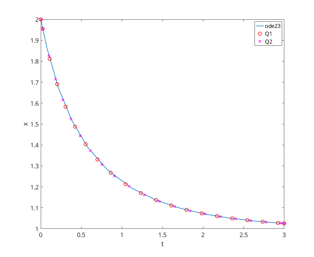
Logistic Equation

figure
[t,x]=ode23(@logistic,[0,3], 2);

plot(t,x(:,1), 'DisplayName', 'ode23');
xlabel('t');
ylabel('x');
hold on;
disp('Logistic Equation:');

tic;
[t,x]=q1_solution(@logistic,0,3, 2);
duration = toc;
plot(t,x(:,1),'ro','DisplayName','Q1');
fprintf('  Q1 Computation Time: %f\n', duration);

tic;
[t,x]=q2_solution(@logistic,0,3, 2);
duration = toc;
plot(t,x(:,1),'mx','DisplayName','Q2');
fprintf('  Q2 Computation Time: %f\n', duration);

legend('Location', 'NorthEast');

Logistic Equation:
  Q1 Computation Time: 0.007764
  Q2 Computation Time: 0.004892

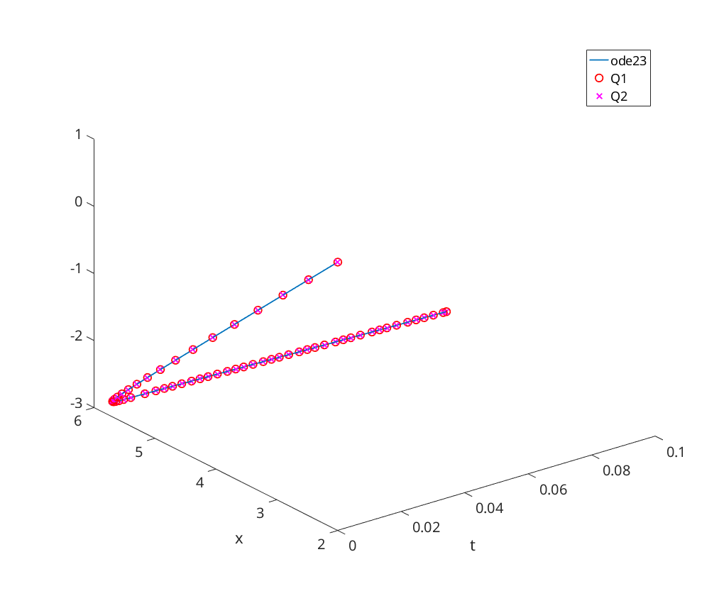
Stiff Linear System

figure
[t,x]=ode23(@linsystem,[0,0.1], [2; 1]);

plot3(t,x(:,1),x(:,2), 'DisplayName', 'ode23');
xlabel('t');
ylabel('x');
hold on;
disp('Stiff Linear System:');

tic;
[t,x]=q1_solution(@linsystem,0,0.1, [2; 1]);
duration = toc;
plot3(t,x(:,1),x(:,2),'ro','DisplayName','Q1');
fprintf('  Q1 Computation Time: %f\n', duration);

tic;
[t,x]=q2_solution(@linsystem,0,0.1, [2; 1]);
duration = toc;
plot3(t,x(:,1),x(:,2),'mx','DisplayName','Q2');
fprintf('  Q2 Computation Time: %f\n', duration);

legend('Location', 'NorthEast');

Stiff Linear System:
  Q1 Computation Time: 0.006402
  Q2 Computation Time: 0.004422

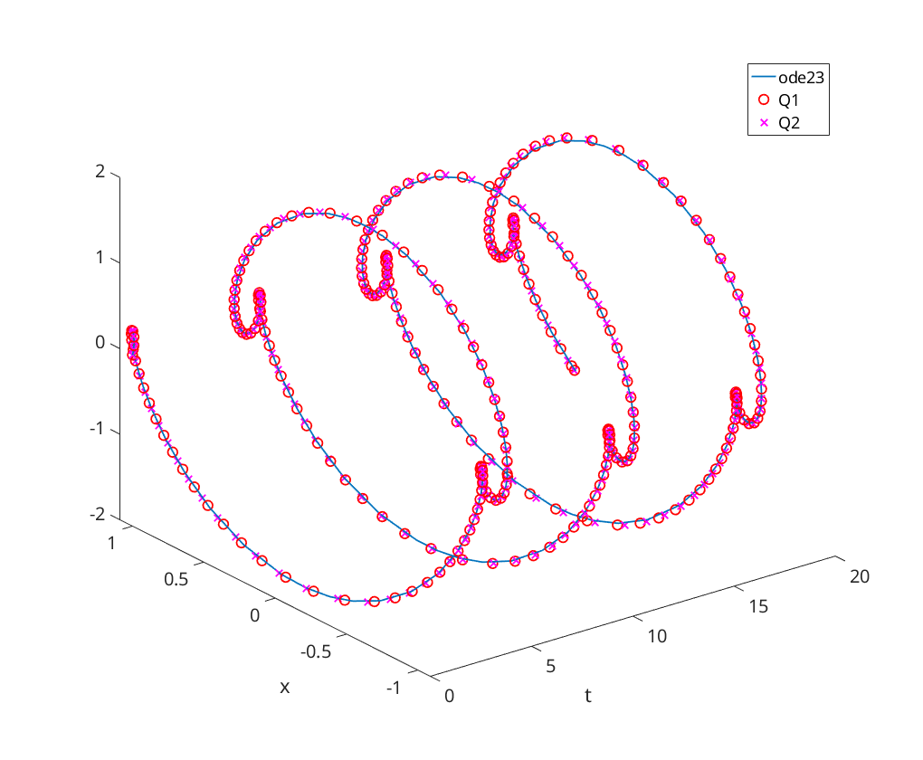
Oscillator

figure
[t,x]=ode23(@oscillator,[0, 20], [1, 0]);

plot3(t,x(:,1),x(:,2), 'DisplayName', 'ode23');
xlabel('t');
ylabel('x');
hold on;
disp('Oscillator:');

tic;
[t,x]=q1_solution(@oscillator,0,20, [1, 0]);
duration = toc;
plot3(t,x(:,1),x(:,2),'ro','DisplayName','Q1');
fprintf('  Q1 Computation Time: %f\n', duration);

tic;
[t,x]=q2_solution(@oscillator,0,20, [1, 0]);
duration = toc;
plot3(t,x(:,1),x(:,2),'mx','DisplayName','Q2');
fprintf('  Q2 Computation Time: %f\n', duration);

legend('Location', 'NorthEast');

Oscillator:
  Q1 Computation Time: 0.005221
  Q2 Computation Time: 0.004245

We note that for Q1 that for the low order method \[\begin{array}{rcl} \kappa_1 &=& f(t,x) \\ \kappa_2 &=& f(t+\tau,x+\tau\kappa_1) \end{array}\] and for the high order method \[\begin{array}{rclcl} \overline\kappa_1 &=& f(t,x) &=& \kappa_1 \\ \overline\kappa_2 &=& f(t+\frac13\tau,x+\frac\tau3\overline\kappa_1) \\ \overline\kappa_3 &=& f(t+\frac23\tau,x+\frac23\tau\overline\kappa_2) \end{array}\] Therefore, four evaluations of $f$ are required.

For Q2, as it is an embedded method, we only have three evaluations of $f$.

We expected that the Q1 method is slower than the Q2 method, which appears to be confirmed by the computation time.

Published with MATLAB® R2023a