Q2 Solution

Contents

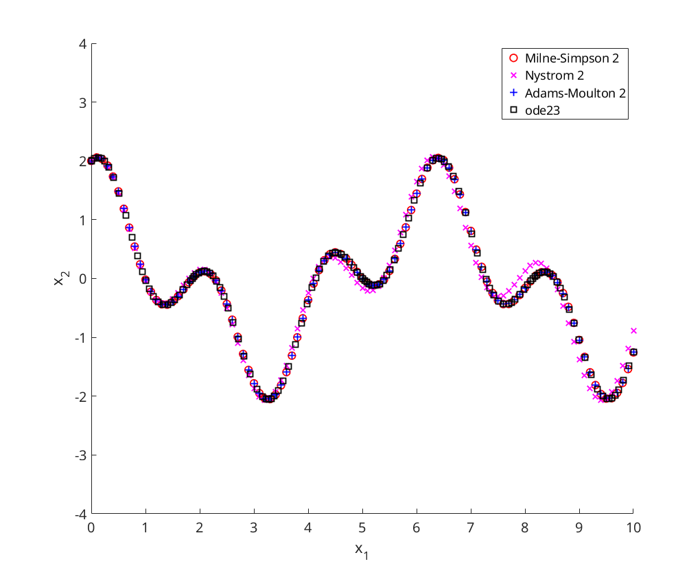
a) Linear Oscillator

We solve linear oscillator with $a = 0$, $b = 9$, $c = 10$, $\omega = 1$ and $x_0=(2,1)^T$ using Milne-Simpson 2, Nystrom 2, Adams-Moulton 2, and ODE23

figure
axis([0 10 -4 4]);
hold on;
xlabel('x_1');
ylabel('x_2');

[t,x]=ms2(@oscillator,0,10, [2;1], .1);
plot(t,x(:,1),'ro','DisplayName','Milne-Simpson 2');

[t,x]=ny2(@oscillator,0,10, [2;1], .1);
plot(t,x(:,1),'mx','DisplayName','Nystrom 2');

[t,x]=am2(@oscillator,0,10, [2;1], .1);
plot(t,x(:,1),'b+','DisplayName','Adams-Moulton 2');

[t,x]=ode23(@oscillator, [0,10], [2;1]);
plot(t,x(:,1),'ks','DisplayName','ode23');

legend('Location', 'NorthEast');

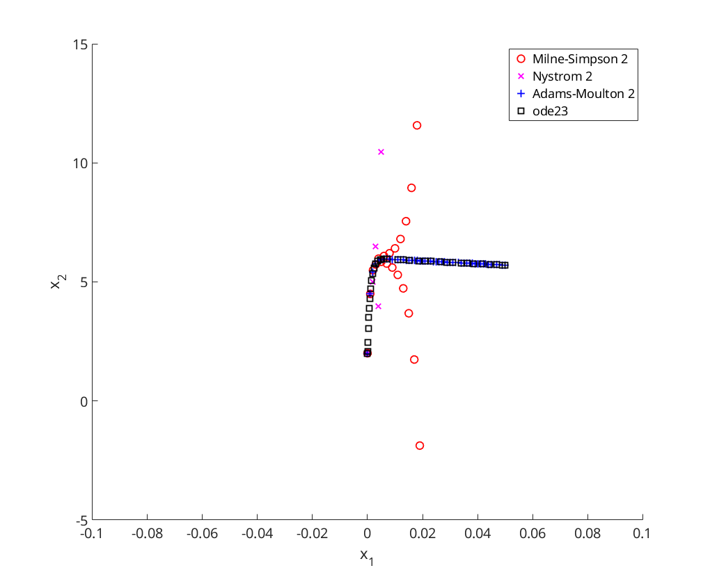
b) Linear System - Adams-Moulton 2-step

We solve the stiff linear system with $x_0=(2,1)^T$ using Milne-Simpson 2, Nystrom 2, Adams-Moulton 2, and ODE23

figure
axis([0 10 -4 4]);
hold on;
xlabel('x_1');
ylabel('x_2');

[t,x]=ms2(@linsystem,0,0.05, [2;1], .001);
plot(t,x(:,1),'ro','DisplayName','Milne-Simpson 2');

[t,x]=ny2(@linsystem,0,0.05, [2;1], .001);
plot(t,x(:,1),'mx','DisplayName','Nystrom 2');

[t,x]=am2(@linsystem,0,0.05, [2;1], .001);
plot(t,x(:,1),'b+','DisplayName','Adams-Moulton 2');

[t,x]=ode23(@linsystem, [0,0.05], [2;1]);
plot(t,x(:,1),'ks','DisplayName','ode23');

ylim([-5 15]);
xlim([-.1 .1]);
legend('Location', 'NorthEast');

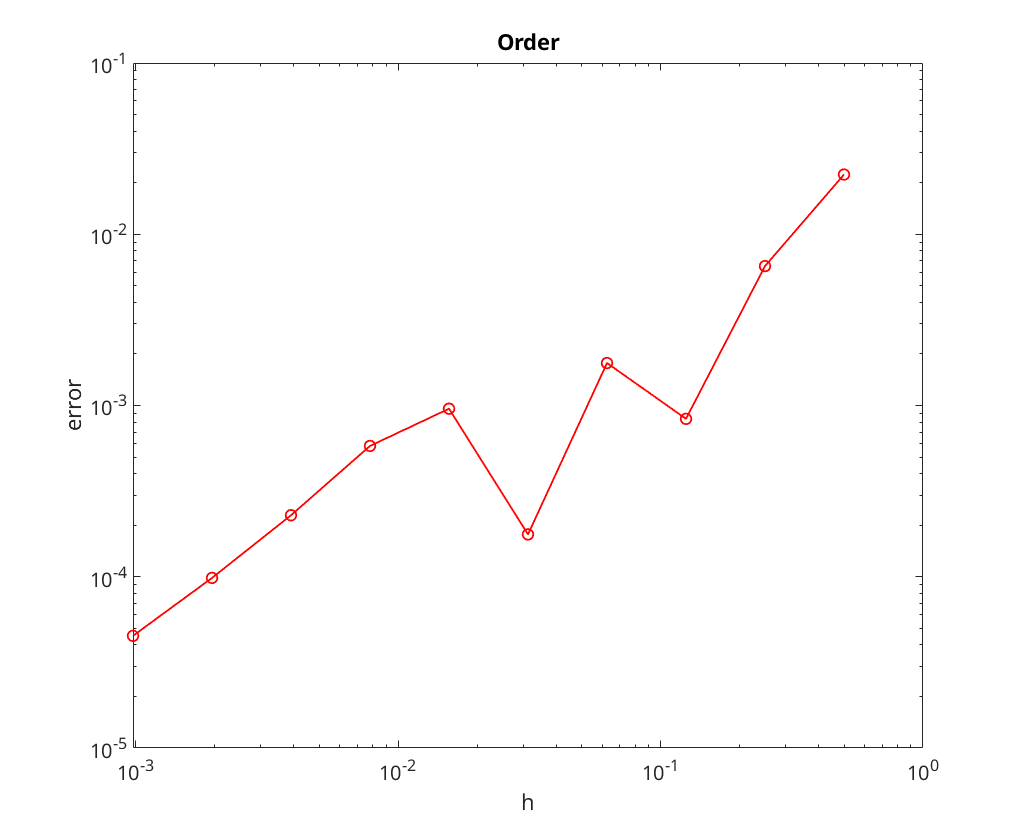
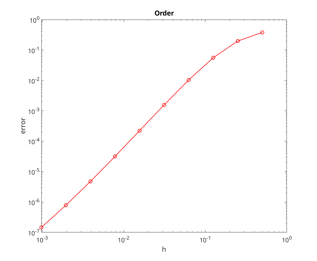
Convergence Analysis for Milne-Simpson and Nystrom

fprintf('Milne-Simpson 2-step = ');
conv_analysis(@ms2);
fprintf('Nystrom 2-step       = ');
conv_analysis(@ny2);

Milne-Simpson 2-step = log_{10}E_N = -1.816019 + 0.815825 x log10(error)
Nystrom 2-step       = log_{10}E_N = 0.781692 + 2.501632 x log10(error)

Published with MATLAB® R2023a