Q1 Solution

Contents

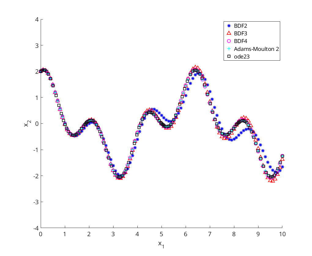
a) Linear Oscillator

We solve linear oscillator with $a = 0$, $b = 9$, $c = 10$, $\omega = 1$ and $x_0=(2,1)^T$ using BDF2, BDF3, BDF4, Adams-Moulton 2, and ODE23

function q3_solution

figure
axis([0 10 -4 4]);
hold on;
xlabel('x_1');
ylabel('x_2');

[t,x]=bdf2(@oscillator,0,10, [2;1], .1);
plot(t,x(:,1),'b*','DisplayName','BDF2');

[t,x]=bdf3(@oscillator,0,10, [2;1], .1);
plot(t,x(:,1),'r^','DisplayName','BDF3');

[t,x]=bdf4(@oscillator,0,10, [2;1], .1, 0.001);
plot(t,x(:,1),'mo','DisplayName','BDF4');

[t,x]=am2(@oscillator,0,10, [2;1], .1);
plot(t,x(:,1),'c+','DisplayName','Adams-Moulton 2');

[t,x]=ode23(@oscillator, [0,10], [2;1]);
plot(t,x(:,1),'ks','DisplayName','ode23');

legend('Location', 'NorthEast');

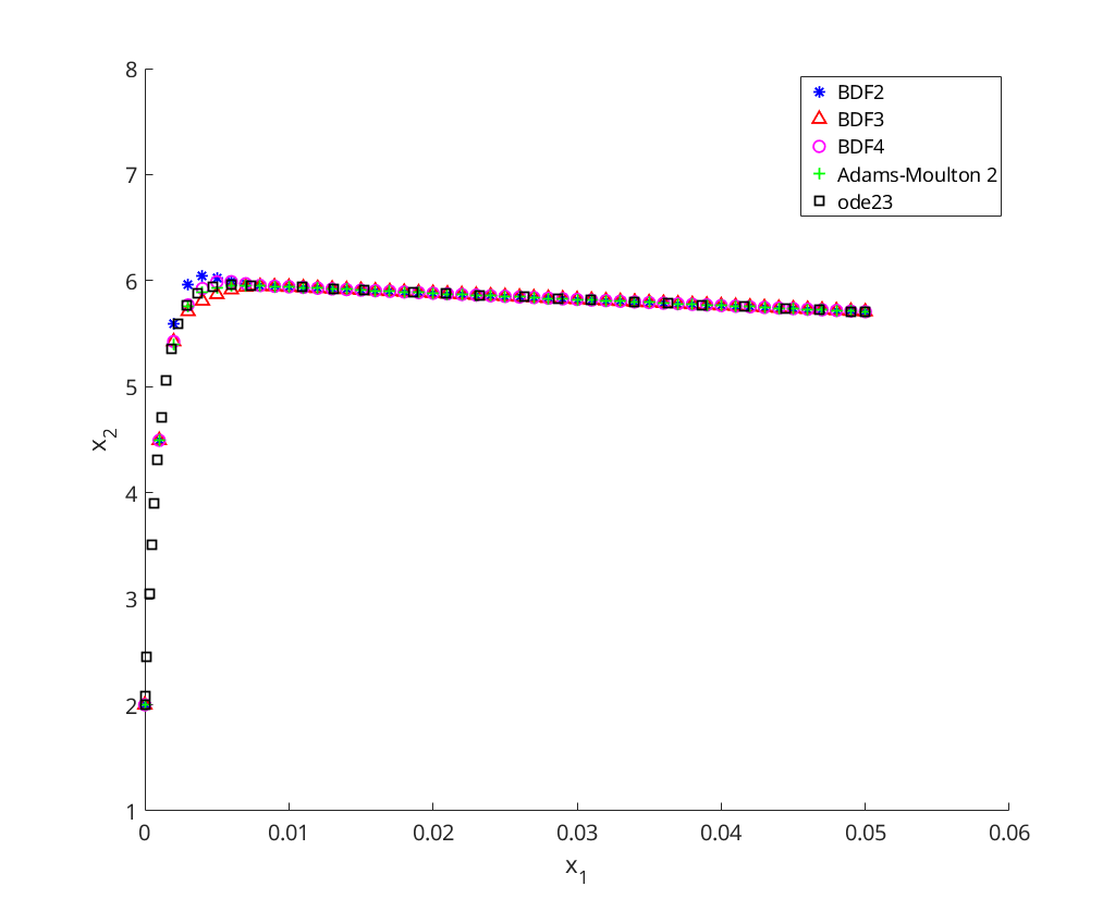
b) Linear System - Adams-Moulton 2-step

We solve the stiff linear system with $x_0=(2,1)^T$ using Adams-Moulton 2, Adams-Moulton 2 with AB2 initial guess, Adams-Bashfort 2, and Adams-Bashfort 3

figure
axis([0 10 -4 4]);
hold on;
xlabel('x_1');
ylabel('x_2');

[t,x]=bdf2(@linsystem,0,0.05, [2;1], .001);
plot(t,x(:,1),'b*','DisplayName','BDF2');

[t,x]=bdf3(@linsystem,0,0.05, [2;1], .001);
plot(t,x(:,1),'r^','DisplayName','BDF3');

[t,x]=bdf4(@linsystem,0,0.05, [2;1], .001, 0.001);
plot(t,x(:,1),'mo','DisplayName','BDF4');

[t,x]=am2(@linsystem,0,0.05, [2;1], .001);
plot(t,x(:,1),'g+','DisplayName','Adams-Moulton 2');

[t,x]=ode23(@linsystem, [0,0.05], [2;1]);
plot(t,x(:,1),'ks','DisplayName','ode23');

ylim([1 8]);
xlim([0 .06]);
legend('Location', 'NorthEast');

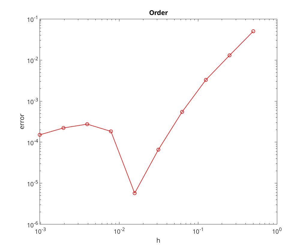
Convergence Analysis for BDF2, BDF3, BDF4

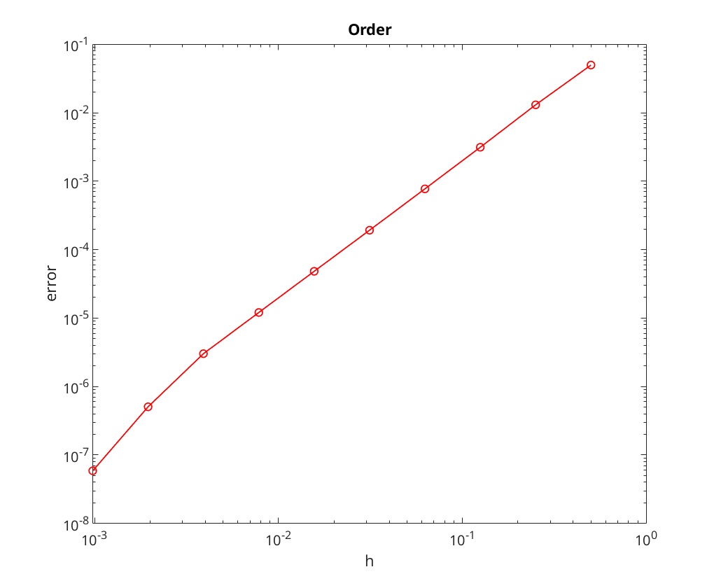
We first perform convergence analysis with the default tolerance of $0.001$

tol = 0.001;
fprintf('BDF2 = ');
conv_analysis(@(field, t0, T, x0, h)bdf2_tol(field, t0, T, x0, h, tol));
fprintf('BDF3 = ');
conv_analysis(@(field, t0, T, x0, h)bdf3_tol(field, t0, T, x0, h, tol));
fprintf('BDF4 = ');
conv_analysis(@(field, t0, T, x0, h)bdf4(field, t0, T, x0, h, tol));

BDF2 = log_{10}E_N = -1.881741 + 0.864464 x log10(error)
BDF3 = log_{10}E_N = -2.175821 + 0.697432 x log10(error)
BDF4 = log_{10}E_N = -2.551904 + 0.547442 x log10(error)

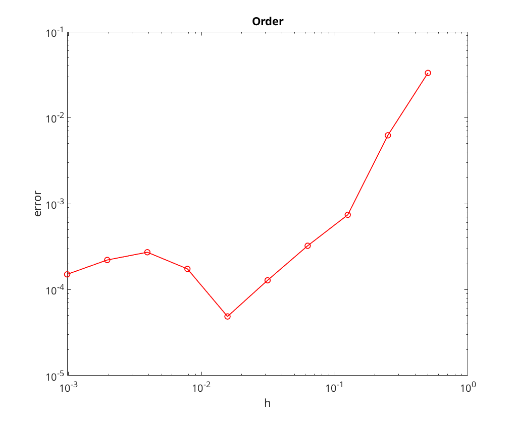
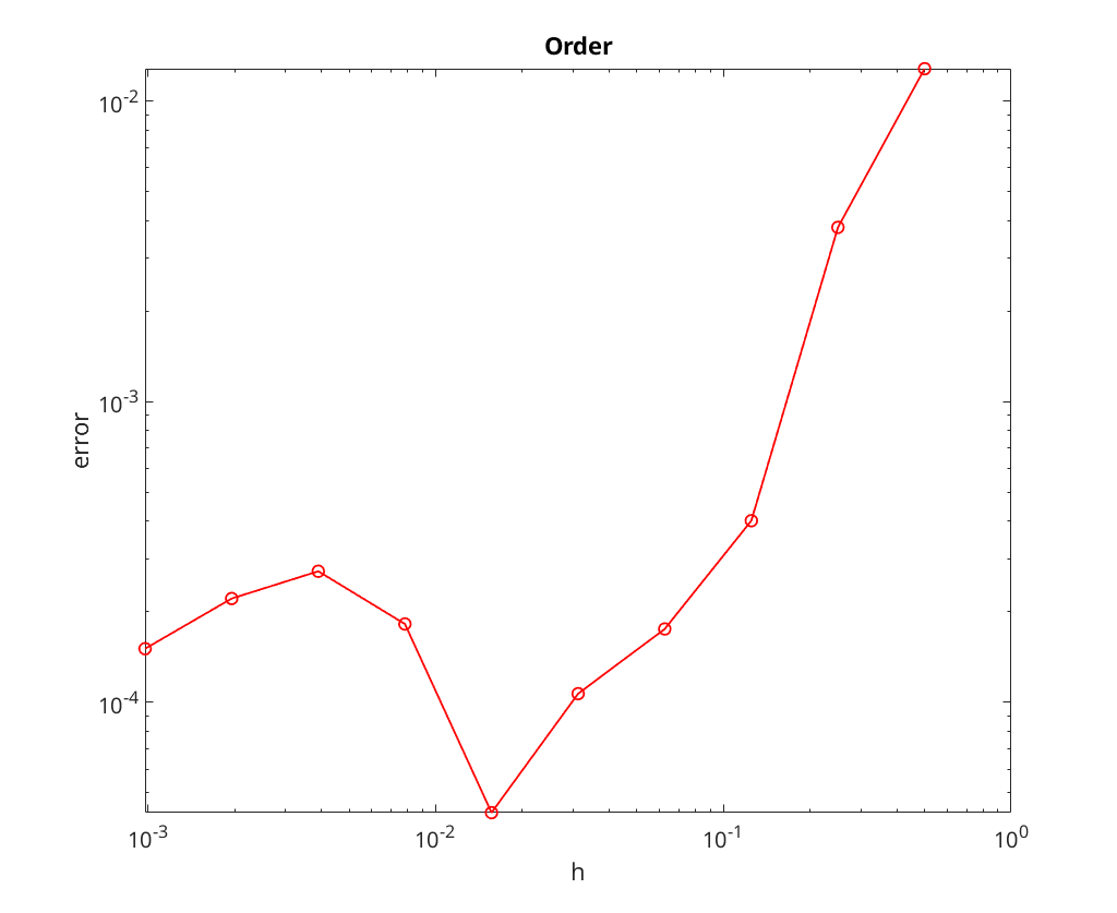
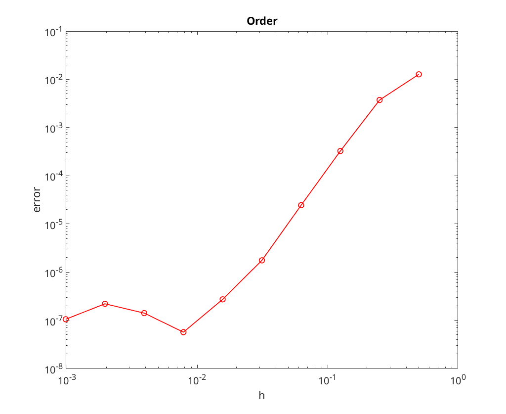
We now perform convergence analysis with a tolerance of $10^{-6}$

tol = 1e-6;
fprintf('BDF2 = ');
conv_analysis(@(field, t0, T, x0, h)bdf2_tol(field, t0, T, x0, h, tol));
fprintf('BDF3 = ');
conv_analysis(@(field, t0, T, x0, h)bdf3_tol(field, t0, T, x0, h, tol));
fprintf('BDF4 = ');
conv_analysis(@(field, t0, T, x0, h)bdf4(field, t0, T, x0, h, tol));

BDF2 = log_{10}E_N = -0.569790 + 2.120640 x log10(error)
BDF3 = log_{10}E_N = -1.220586 + 2.193145 x log10(error)
BDF4 = log_{10}E_N = -1.885049 + 2.030965 x log10(error)

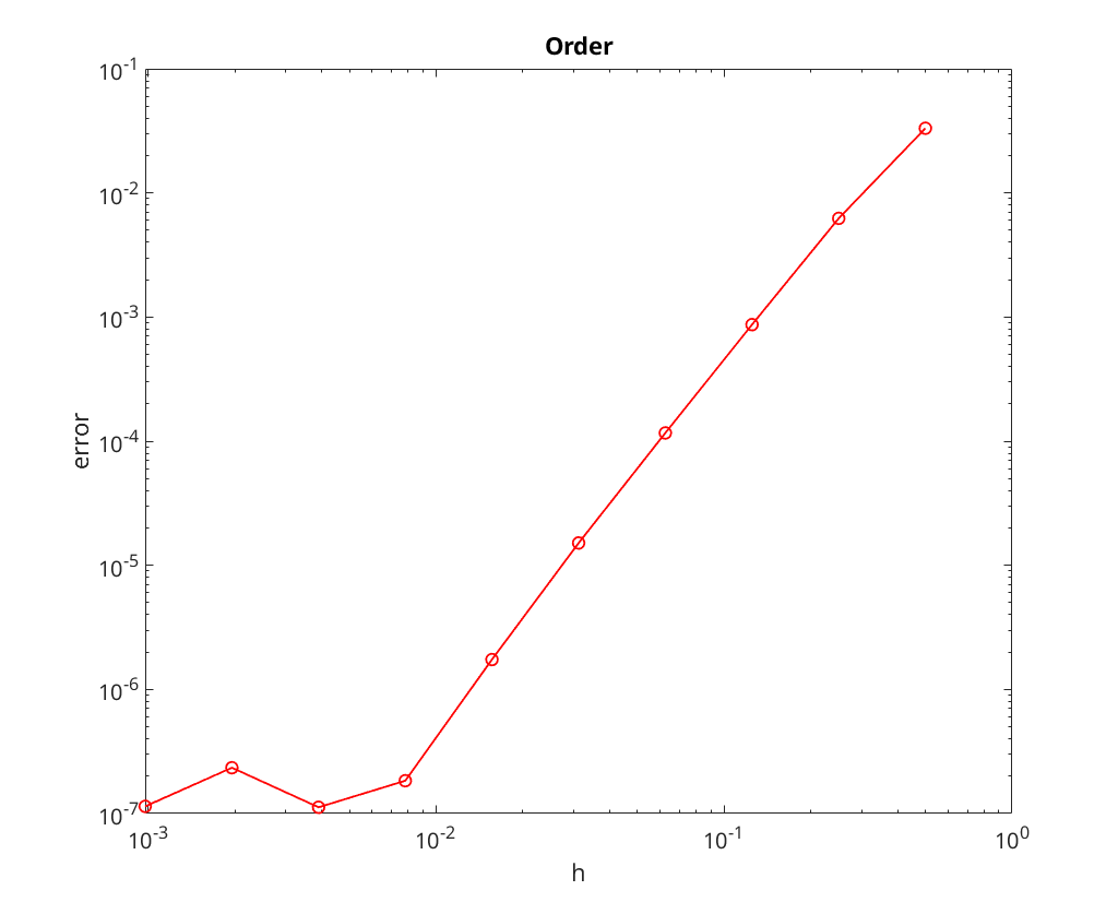
Finally we perform convergence analysis with a tolerance of $10^{-10}$

tol = 1e-10;
fprintf('BDF2 = ');
conv_analysis(@(field, t0, T, x0, h)bdf2_tol(field, t0, T, x0, h, tol));
fprintf('BDF3 = ');
conv_analysis(@(field, t0, T, x0, h)bdf3_tol(field, t0, T, x0, h, tol));
fprintf('BDF4 = ');
conv_analysis(@(field, t0, T, x0, h)bdf4(field, t0, T, x0, h, tol));

BDF2 = log_{10}E_N = -0.693351 + 2.005649 x log10(error)
BDF3 = log_{10}E_N = -0.461389 + 2.929519 x log10(error)
BDF4 = log_{10}E_N = -0.498977 + 3.550965 x log10(error)

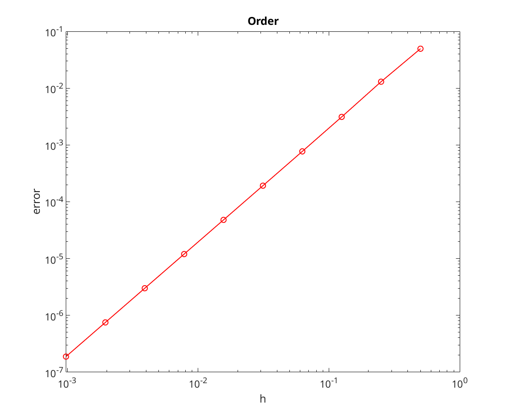
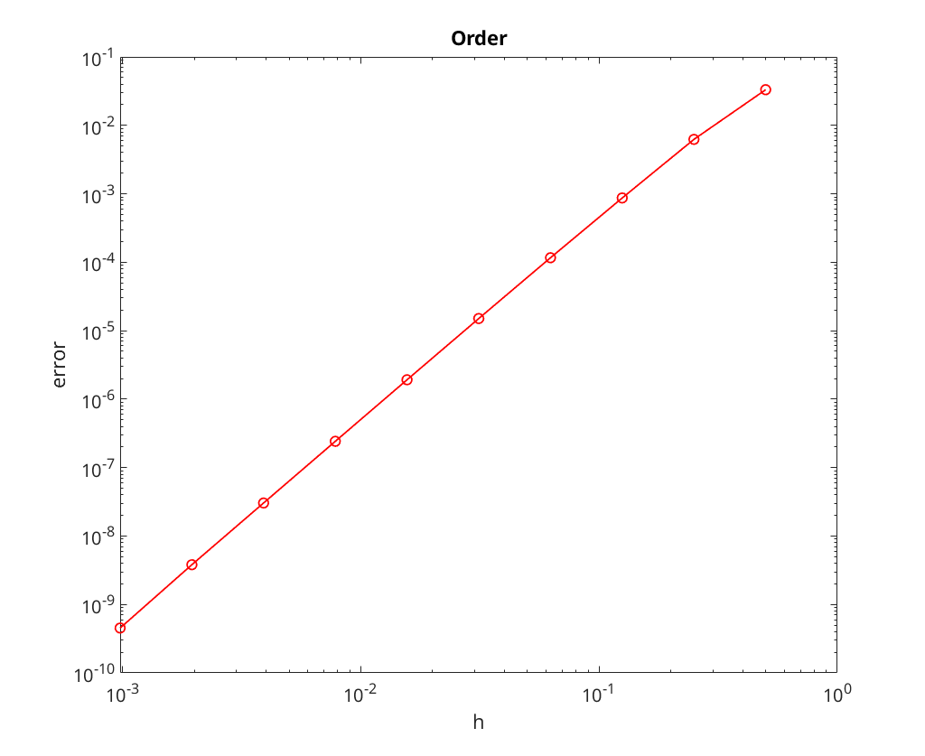
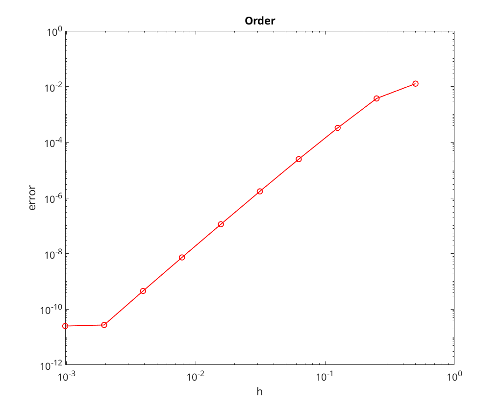
We note that the convergence rate seems to be limited by the tolerance for the nonlinear solve; most notable, look at the plots the method appears to stop converging once the error is down to roughly the tolerance level.

BDF4 Implementation

function [t,x] = bdf4(field, t0, T, x0, h, tol)

m = 4;
n = ceil((T-t0)/h);

t = t0+h*(0:n).';
x = ones(n+1,length(x0));
[to,xo] = rk_classical(field, t0, t0+(m-1)*h, x0, h);
t(1:m) = to(1:m);
x(1:m,:) = xo(1:m,:);

for i=m:n
    f_old = feval(field, t(i)+h, x(i,:).');
    x(i+1,:) = (48*x(i,:).' - 36*x(i-1,:).' + 16*x(i-2,:).' ...
        - 3*x(i-3,:).' + 12*h*f_old)/25;
    f_new = feval(field, t(i)+h, x(i+1,:).');
    while norm(f_old-f_new, 'inf') >= tol
        f_old = f_new;
        x(i+1,:) = (48*x(i,:).' - 36*x(i-1,:).' + 16*x(i-2,:).' ...
            - 3*x(i-3,:).' + 12*h*f_old)/25;
        f_new = feval(field, t(i)+h, x(i+1,:).');
    end
end

end

BDF3 Implementation (with Tolerance)

function [t,x] = bdf3_tol(field, t0, T, x0, h, tol)

m = 3;
n = ceil((T-t0)/h);

t = t0+h*(0:n).';
x = ones(n+1,length(x0));
[to,xo] = rk_classical(field, t0, t0+(m-1)*h, x0, h);
t(1:m) = to(1:m);
x(1:m,:) = xo(1:m,:);

for i=m:n
    f_old = feval(field, t(i)+h, x(i,:).');
    x(i+1,:) = (18*x(i,:).' - 9*x(i-1,:).' + 2*x(i-2,:).' + 6*h*f_old)/11;
    f_new = feval(field, t(i)+h, x(i+1,:).');
    while norm(f_old-f_new, 'inf') >= tol
        f_old = f_new;
        x(i+1,:) = (18*x(i,:).' - 9*x(i-1,:).' + 2*x(i-2,:).' + 6*h*f_old)/11;
        f_new = feval(field, t(i)+h, x(i+1,:).');
    end
end
end

BDF2 Implementation (with Tolerance)

function [t,x] = bdf2_tol(field, t0, T, x0, h, tol)

m = 2;
n = ceil((T-t0)/h);

t = t0+h*(0:n).';
x = ones(n+1,length(x0));
[to,xo] = rk_classical(field, t0, t0+(m-1)*h, x0, h);
t(1:m) = to(1:m);
x(1:m,:) = xo(1:m,:);

for i=m:n
    f_old = feval(field, t(i)+h, x(i,:).');
    x(i+1,:) = (4*x(i,:).' - x(i-1,:).' + 2*h*f_old)/3;
    f_new = feval(field, t(i)+h, x(i+1,:).');
    while norm(f_old-f_new, 'inf') >= tol
        f_old = f_new;
        x(i+1,:) = (4*x(i,:).' - x(i-1,:).' + 2*h*f_old)/3;
        f_new = feval(field, t(i)+h, x(i+1,:).');
    end
end
end

end

Published with MATLAB® R2023a