Stokes equation

Stokes flow around cylinder

Solve the following linear system of PDEs

\[\begin{split}- \operatorname{div}(\nabla u) + \nabla p &= f \quad\text{ in }\Omega, \\ \operatorname{div} u &= 0 \quad\text{ in }\Omega, \\ u &= 0 \quad\text{ on }\Gamma_\mathrm{D}, \\ u &= u_\mathrm{IN} \quad\text{ on }\Gamma_\mathrm{IN}, \\ \tfrac{\partial u}{\partial\mathbf{n}} &= g \quad\text{ on }\Gamma_\mathrm{N}, \\\end{split}\]

using FE discretization with data

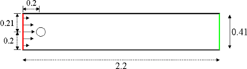
• \(\Omega = [0, 2.2]x[0, 0.41] - B_{0.05}\left([0.2,0.2]\right)\)
• \(\Gamma_\mathrm{N} = \left\{ x = 2.2 \right\}\)
• \(\Gamma_\mathrm{IN} = \left\{ x = 0.0 \right\}\)
• \(\Gamma_\mathrm{D} = \Gamma_\mathrm{W} \cup \Gamma_\mathrm{S}\)
• \(u_\mathrm{IN} = \left( 0.3 \frac{4}{0.41^2} y (0.41-y) , 0 \right)\)

where \(B_R(\mathbf{z})\) is a circle of radius \(R\) and center \(\mathbf{z}\)

Task 1. Write the variational formulation of the problem and discretize the equation by mixed finite element method.

Task 2. Build mesh, prepare facet function marking \(\Gamma_\mathrm{N}\) and \(\Gamma_\mathrm{D}\) and plot it to check its correctness.

Hint. Use the mshr component of fenics - see mshr documentation

import mshr

# Define domain
center = Point(0.2, 0.2)
radius = 0.05
L = 2.2
W = 0.41
geometry =  mshr.Rectangle(Point(0.0,0.0), Point(L, W)) \
           -mshr.Circle(center, radius, 10)

# Build mesh
mesh = mshr.generate_mesh(geometry, 50)

Hint. Try yet another way to mark the boundaries by direct access to the mesh entities by facets(mehs), vertices(mesh), cells(mesh)

# Construct facet markers
bndry = FacetFunction("size_t", mesh)
for f in facets(mesh):
     mp = f.midpoint()
     if near(mp[0], 0.0): bndry[f] = 1  # inflow
     elif near(mp[0], L): bndry[f] = 2  # outflow
     elif near(mp[1], 0.0) or near(mp[1], W): bndry[f] = 3  # walls
     elif mp.distance(center) <= radius:      bndry[f] = 5  # cylinder

plot(boundary_parts, interactive=True)

Task 3. Construct the mixed finite element space and the bilinear and linear forms together with the DirichletBC object.

Hint. Use for example the stable Taylor-Hood finite elements.

# Build function spaces (Taylor-Hood)
V = VectorFunctionSpace(mesh, "Lagrange", 2)
P = FunctionSpace(mesh, "Lagrange", 1)
W = MixedFunctionSpace([V, P])

Hint. To define Dirichlet BC on subspace use the W.sub method.

noslip = Constant((0, 0))
bc_walls = DirichletBC(W.sub(0), noslip, bndry, 3)

Hint. To build the forms use the split method or function to access the components of the mixed space.

# Define unknown and test function(s)
(v_, p_) = TestFunctions(W)
(v , p)  = TrialFunctions(W)

Then you can define the forms for example as:

def a(u,v): return inner(grad(u), grad(v))*dx
def b(p,v): return p*div(v)*dx
def L(v):   return inner(f, v)*dx

F = a(v,v_) + b(p,v_) + b(p_,v) - L(v_)

And solve by:

w = Function(W)
solve(lhs(F)==rhs(F), w, bcs)
(v,p)=w.split(w)

Task 4. Now modify the problem to the Navier-Stokes equations and compute the DFG-flow around cylinder benchmark

Hint. You can use generic solve function or NonlinearVariationalProblem and NonlinearVariationalSolver classes.

(_v, _p) = TestFunctions(W)
w = Function(W)
(v, p) = split(w)

I = Identity(v.geometric_dimension())    # Identity tensor

D = 0.5*(grad(v)+grad(v).T)  # or D=sym(grad(v))
T = -p*I + 2*nu*D

# Define variational forms
F = inner(T, grad(_v))*dx + _p*div(v)*dx + inner(grad(v)*v,_v)*dx

Hint. Use Assemble function to evaluate the lift and drag functionals.

force = T*n
D = (force[0]/0.002)*ds(5)
L = (force[1]/0.002)*ds(5)

drag = assemble(D)
lift = assemble(L)

print "drag= %e    lift= %e" % (drag , lift)

Task 5. Now prepare the time dependent solution of the Navier-Stokes equations. Combine it with the heat equation example.

Reference solution

from dolfin import *
import mshr

# Define domain
center = Point(0.2, 0.2)
radius = 0.05
L = 2.2
W = 0.41
geometry = mshr.Rectangle(Point(0.0, 0.0), Point(L, W)) \
         - mshr.Circle(center, radius, 10)

# Build mesh
mesh = mshr.generate_mesh(geometry, 50)

# Construct facet markers
bndry = FacetFunction("size_t", mesh)
for f in facets(mesh):
    mp = f.midpoint()
    if near(mp[0], 0.0): # inflow
        bndry[f] = 1
    elif near(mp[0], L): # outflow
        bndry[f] = 2
    elif near(mp[1], 0.0) or near(mp[1], W): # walls
        bndry[f] = 3
    elif mp.distance(center) <= radius: # cylinder
        bndry[f] = 5

# Build function spaces (Taylor-Hood)
V = VectorFunctionSpace(mesh, "CG", 2)
P = FunctionSpace(mesh, "CG", 1)
W = MixedFunctionSpace([V, P])

# No-slip boundary condition for velocity on walls and cylinder - boundary id 3
noslip = Constant((0, 0))
bc_walls = DirichletBC(W.sub(0), noslip, bndry, 3)
bc_cylinder = DirichletBC(W.sub(0), noslip, bndry, 5)

# Inflow boundary condition for velocity - boundary id 1
v_in = Expression(("0.3 * 4.0 * x[1] * (0.41 - x[1]) / ( 0.41 * 0.41 )", "0.0"))
bc_in = DirichletBC(W.sub(0), v_in, bndry, 1)

# Collect boundary conditions
bcs = [bc_cylinder, bc_walls, bc_in]

# Facet normal, identity tensor and boundary measure
n = FacetNormal(mesh)
I = Identity(mesh.geometry().dim())
ds = Measure("ds", subdomain_data=bndry)
nu = Constant(0.001)


def stokes():

    # Define variational forms for Stokes
    def a(u,v):
        return inner(nu*grad(u), grad(v))*dx
    def b(p,v):
        return p*div(v)*dx
    def L(v):
        return inner(Constant((0.0,0.0)), v)*dx

    # Solve the problem
    u, p = TrialFunctions(W)
    v, q = TestFunctions(W)
    w = Function(W)
    solve(a(u, v) - b(p, v) - b(q, u) == L(v), w, bcs)

    # Report in,out fluxes
    u = w.sub(0, deepcopy=False)
    info("Inflow flux:  %e" % assemble(inner(u, n)*ds(1)))
    info("Outflow flux: %e" % assemble(inner(u, n)*ds(2)))

    return w


def navier_stokes():

    v, q = TestFunctions(W)
    w = Function(W)
    u, p = split(w)

    # Define variational forms
    T = -p*I + 2.0*nu*sym(grad(u))
    F = inner(T, grad(v))*dx - q*div(u)*dx + inner(grad(u)*u, v)*dx

    solve(F == 0, w, bcs)

    # Report drag and lift
    force = dot(T, n)
    D = (force[0]/0.002)*ds(5)
    L = (force[1]/0.002)*ds(5)
    drag = assemble(D)
    lift = assemble(L)
    info("drag= %e    lift= %e" % (drag , lift))

    # Report pressure difference
    a_1 = Point(0.15, 0.2)
    a_2 = Point(0.25, 0.2)
    p = w.sub(1, deepcopy=False)
    p_diff = p(a_1) - p(a_2)
    info("p_diff = %e" % p_diff)

    return w


if __name__ == "__main__":

    for problem in [stokes, navier_stokes]:
        begin("Running '%s'" % problem.__name__)

        # Call solver
        w = problem()

        # Extract solutions
        u, p = w.split()

        # Save solution
        ufile = File("results_%s/u.xdmf" % problem.__name__)
        pfile = File("results_%s/p.xdmf" % problem.__name__)
        u.rename("u", "velocity")
        p.rename("p", "pressure")
        ufile << u
        pfile << p

        plot(u, title='velocity %s' % problem.__name__)
        plot(p, title='pressure %s' % problem.__name__)

        end()

    interactive()

Navier-Stokes + convection-difusion

from dolfin import *
import mshr

comm = mpi_comm_world()
rank = MPI.rank(comm)
set_log_level(INFO if rank==0 else INFO+1)
parameters["std_out_all_processes"] = False

# Define domain
center = Point(0.2, 0.2)
radius = 0.05
L = 2.2
W = 0.41
geometry = mshr.Rectangle(Point(0.0, 0.0), Point(L, W)) \
         - mshr.Circle(center, radius, 10)

# Build mesh
mesh = mshr.generate_mesh(geometry, 50)

# Construct facet markers
bndry = FacetFunction("size_t", mesh)
for f in facets(mesh):
    mp = f.midpoint()
    if near(mp[0], 0.0): # inflow
        bndry[f] = 1
    elif near(mp[0], L): # outflow
        bndry[f] = 2
    elif near(mp[1], 0.0) or near(mp[1], W): # walls
        bndry[f] = 3
    elif mp.distance(center) <= radius: # cylinder
        bndry[f] = 5

# Build function spaces (Taylor-Hood)
V = VectorFunctionSpace(mesh, "CG", 2)
P = FunctionSpace(mesh, "CG", 1)
E = FunctionSpace(mesh, "CG", 1)
W = MixedFunctionSpace([V, P, E])

# No-slip boundary condition for velocity on walls and cylinder - boundary id 3
noslip = Constant((0, 0))
bcv_walls = DirichletBC(W.sub(0), noslip, bndry, 3)

vc= Expression(("-0.5*t*cos(atan2(x[0]-0.2,x[1]-0.2))","0.5*t*sin(atan2(x[0]-0.2,x[1]-0.2))"),t=0)
bcv_cylinder = DirichletBC(W.sub(0), vc, bndry, 5)

bce_cylinder = DirichletBC(W.sub(2), Constant(1.0), bndry, 5)
# Inflow boundary condition for velocity - boundary id 1
v_in = Expression(("1.5 * 4.0 * x[1] * (0.41 - x[1]) / ( 0.41 * 0.41 )", "0.0"))
bcv_in = DirichletBC(W.sub(0), v_in, bndry, 1)

# Collect boundary conditions
bcs = [bcv_cylinder, bcv_walls, bcv_in, bce_cylinder]

# Facet normal, identity tensor and boundary measure
n = FacetNormal(mesh)
I = Identity(mesh.geometry().dim())
ds = Measure("ds", subdomain_data=bndry)
nu = Constant(0.001)

dt = 0.1
t_end = 10
theta=0.5   # Crank-Nicholson timestepping
k=0.01

# Define unknown and test function(s)
(v_, p_, e_) = TestFunctions(W)

# current unknown time step
w = Function(W)
(v, p, e) = split(w)

# previous known time step
w0 = Function(W)
(v0, p0, e0) = split(w0)

def a(v,u) :
    D = sym(grad(v))
    return (inner(grad(v)*v, u) + inner(2*nu*D, grad(u)))*dx

def b(q,v) :
    return inner(div(v),q)*dx

def c(v,e,g) :
    return ( inner(k*grad(e),grad(g)) + inner(v,grad(e))*g )*dx

# Define variational forms without time derivative in previous time
F0_eq1 = a(v0,v_) + b(p,v_)
F0_eq2 = b(p_,v)
F0_eq3 = c(v0,e0,e_)
F0 = F0_eq1 + F0_eq2 + F0_eq3

# variational form without time derivative in current time
F1_eq1 = a(v,v_) + b(p,v_)
F1_eq2 = b(p_,v)
F1_eq3 = c(v,e,e_)
F1 = F1_eq1 + F1_eq2 + F1_eq3

#combine variational forms with time derivative
#
#  dw/dt + F(t) = 0 is approximated as
#  (w-w0)/dt + (1-theta)*F(t0) + theta*F(t) = 0
#
F = (inner((v-v0),v_)/dt + inner((e-e0),e_)/dt)*dx + (1.0-theta)*F0 + theta*F1

# Create files for storing solution
name="a"
vfile = XDMFFile(mpi_comm_world(),"results_%s/v.xdmf" % name)
pfile = XDMFFile(mpi_comm_world(),"results_%s/p.xdmf" % name)
efile = XDMFFile(mpi_comm_world(),"results_%s/e.xdmf" % name)
vfile.parameters["flush_output"] = True
pfile.parameters["flush_output"] = True
efile.parameters["flush_output"] = True


J = derivative(F, w)
problem=NonlinearVariationalProblem(F,w,bcs,J)
solver=NonlinearVariationalSolver(problem)

prm = solver.parameters
#info(prm,True)  #get full info on the parameters
prm['nonlinear_solver'] = 'newton'
prm['newton_solver']['absolute_tolerance'] = 1E-12
prm['newton_solver']['relative_tolerance'] = 1e-12
prm['newton_solver']['maximum_iterations'] = 20
prm['newton_solver']['linear_solver'] = 'mumps'


# Time-stepping
t = dt
while t < t_end:

    print "t =", t
    #vc.t=t

    # Compute
    begin("Solving ....")
    solver.solve()
    end()

    # Extract solutions:
    (v, p, e) = w.split()

    v.rename("v", "velocity")
    p.rename("p", "pressure")
    e.rename("e", "temperature")
    # Save to file
    vfile << v
    pfile << p
    efile << e

    # Move to next time step
    w0.assign(w)
    t += dt