Hamiltonian Monte Carlo with RStan
Jan Vávra
Download the source code as:
In previous part we have shown that Random-walk Metropolis-Hastings algorithm for sampling Markov chain to explore the posterior distribution is universal to any problem, but tuning the parameters of the proposal distribution is crucial for reasonable acceptance and exploration in practice. Stan is a software available in many interfaces, such as R (Rstan) or Python (Pystan), which boosts the sampling by upgrading to Hamiltonian Monte Carlo and by automatic parameter tuning.
Hamiltonian Monte Carlo
Details about this technique can be read in Rstan reference manual and source literature, e.g. A Conceptual Introduction to Hamiltonian Monte Carlo by Michael Betancourt.. We will only explain the core idea and illustrate its manual implementation on toy example.
Consider a problem of \(D\)-dimensional vector of parameters \(\boldsymbol{\theta}\) with posterior distribution \(p(\boldsymbol{\theta} \,|\, \mathsf{data}) \propto p(\mathsf{data} \,|\, \boldsymbol{\theta}) \; p(\boldsymbol{\theta})\) known up to a multiplicative constant to be explored. The parametric model is extended by parameter \(\boldsymbol{\rho}\) of the same dimension \(D\) sampled independently of \(\boldsymbol{\theta}\): \[ \boldsymbol{\rho} \sim \mathsf{N}_D\left(\boldsymbol{0}, \Sigma\right). \] Previously, we treated \(\boldsymbol{\rho}\) as incremental step to be added to current value of \(\boldsymbol{\theta}\). Here \(\boldsymbol{\rho}\) is treated as momentum variable that navigates us through the parametric space.
The proposal for a new value in Hamiltonian Monte Carlo are given by following the numerical solution of Hamilton’s differential equation: \[ \frac{\mathrm{d}\boldsymbol{\theta}}{\mathrm{d} t} = - \log p (\boldsymbol{\rho}) \qquad \text{and} \qquad \frac{\mathrm{d}\boldsymbol{\rho}}{\mathrm{d} t} = + \log p (\boldsymbol{\theta} \,|\, \mathsf{data}) \] with unknown curves \(\boldsymbol{\theta}(t)\) and \(\boldsymbol{\rho}(t)\) for \(t \in (0, T)\). This interval is cut into smaller intervals of length \(\varepsilon>0\). The numerical solution to these equations takes the initial values \(\boldsymbol{\theta}_0\) and \(\boldsymbol{\rho_0}\) and updates them in \(L\) leapfrog steps: \[ \begin{align} \boldsymbol{\rho}_{l+\frac{1}{2}} \quad&\longleftarrow\quad \boldsymbol{\rho}_l + \frac{\varepsilon}{2} \left.\frac{\partial \log p (\boldsymbol{\theta} \,|\, \mathsf{data})}{\partial \boldsymbol{\theta}}\right|_{\boldsymbol{\theta} = \boldsymbol{\theta}_l}; \\ \boldsymbol{\theta}_{l+1} \quad&\longleftarrow\quad \boldsymbol{\theta}_l - \varepsilon \left.\frac{\partial \log p (\boldsymbol{\rho})}{\partial \boldsymbol{\rho}}\right|_{\boldsymbol{\rho} = \boldsymbol{\rho}_{l+\frac{1}{2}}} = \boldsymbol{\theta}_l + \varepsilon \Sigma^{-1} \boldsymbol{\rho}_{l+\frac{1}{2}}; \\ \boldsymbol{\rho}_{l+1} \quad&\longleftarrow\quad \boldsymbol{\rho}_{l+\frac{1}{2}} + \frac{\varepsilon}{2} \left.\frac{\partial \log p (\boldsymbol{\theta} \,|\, \mathsf{data})}{\partial \boldsymbol{\theta}}\right|_{\boldsymbol{\theta} = \boldsymbol{\theta}_{l+1}}. \end{align} \] After these \(L\) steps we have \(\boldsymbol{\theta_L}\) and \(\boldsymbol{\rho_L}\) - the proposal candidates for Metropolis-Hastings part.
The design of these steps does not fulfill the reversibility condition so additional step that negates the momentum \(\boldsymbol{\rho}\) has to be added. This way the transition density from \((\boldsymbol{\theta}_0, \boldsymbol{\rho}_0)\) to \((\boldsymbol{\theta}_L, \boldsymbol{\rho}_L)\) and from \((\boldsymbol{\theta}_L, \boldsymbol{\rho}_L)\) to \((\boldsymbol{\theta}_0, \boldsymbol{\rho}_0)\) are equal. so the computation of the acceptance probability reduces to \[ \min \left\{1, \quad \exp\left[ \log p(\boldsymbol{\theta}_L \,|\, \mathsf{data}) + \log p(\boldsymbol{\rho}_L) - \log p(\boldsymbol{\theta}_0 \,|\, \mathsf{data}) - \log p(\boldsymbol{\rho}_0) \right]\right\}. \] With this probability \(\boldsymbol{\theta}_L\) is accepted as new value for \(\boldsymbol{\theta}\), otherwise the chain stays in \(\boldsymbol{\theta}_0\). The momentum variable \(\boldsymbol{\rho}\) is forgotten. Let’s demonstrate the use on simple example.
Example - \(\mathsf{N}(\mu, \sigma_0^2)\) with \(\sigma_0\) known
Let us have a random sample \(Y_1, \ldots, Y_n \sim \mathsf{N}(\mu, \sigma_0^2)\) where \(\mu \in \mathbb{R}\) is unknown model parameter.
set.seed(123456789)
n <- 50
sigma02 <- 1
data <- rnorm(n, mean = 10, sd = sqrt(sigma02))
mean(data)
## [1] 9.843967Then, the model contribution to the posterior is \[ \log p (Y_1, \ldots, Y_n \,|\, \mu) = \mathrm{const} -\frac{1}{2\sigma_0^2} \sum\limits_{i=1}^n (Y_i - \mu)^2 = \mathrm{const} -\frac{n}{2\sigma_0^2} (\mu^2 - 2\mu \overline{Y}_n). \] Assuming normal prior \(\mu \sim \mathsf{N}(\mu_\mu, \sigma_\mu^2)\) we get the following posterior log-density: \[ \begin{align} \log p(\mu \,|\, Y_1, \ldots, Y_n) &= \mathrm{const} -\frac{n}{2\sigma_0^2} (\mu^2 - 2\mu \overline{Y}_n) - \frac{1}{2\sigma_\mu^2} (\mu - \mu_\mu)^2, \\ \frac{\partial \log p(\mu \,|\, Y_1, \ldots, Y_n)}{\partial \mu} &= \frac{n \overline{Y}_n}{\sigma_0^2} + \frac{\mu_\mu}{\sigma_\mu^2} - \mu \left(\frac{n}{\sigma_0^2} + \frac{1}{\sigma_\mu^2}\right), \end{align} \] which we know to be the log-density of normal distribution.
mumu <- 5
sigmamu2 <- 100
How would look the iterative algorithm to reach a proposal in this case?
Assume \(\rho \sim \mathsf{N}(0, \sigma_\rho^2)\).
sigmarho2 <- 1Then, given initial values \(\mu_0\) and \(\rho_0\) we get the following updates: \[ \begin{align} \rho_{l+\frac{1}{2}} \quad&\longleftarrow\quad \rho_l + \frac{\varepsilon}{2} \left[\frac{n \overline{Y}_n}{\sigma_0^2} + \frac{\mu_\mu}{\sigma_\mu^2} - \mu_l \left(\frac{n}{\sigma_0^2} + \frac{1}{\sigma_\mu^2}\right)\right]; \\ \mu_{l+1} \quad&\longleftarrow\quad \mu_l + \varepsilon \frac{\rho_{l+\frac{1}{2}}}{\sigma_\rho^2}; \\ \rho_{l+1} \quad&\longleftarrow\quad \rho_{l+\frac{1}{2}} + \frac{\varepsilon}{2} \left[\frac{n \overline{Y}_n}{\sigma_0^2} + \frac{\mu_\mu}{\sigma_\mu^2} - \mu_{l+1} \left(\frac{n}{\sigma_0^2} + \frac{1}{\sigma_\mu^2}\right)\right]. \end{align} \] This is the manual implementation that even tracks the changes in between (just for illustration):
leapfrog_path_example <- function(data, rho0, mu0, L = 10, eps = 0.01, sigmarho2 = 1, sigma02 = 1, mumu = 5, sigmamu2 = 100){
  rho <- rho1 <- rho2 <- mu <- as.numeric(L+1)
  rho[1] <- rho1[1] <- rho2[1] <- rho0
  mu[1] <- mu0
  post_prec <- length(data)/sigma02 + 1/sigmamu2
  post_mean <- (sum(data) / sigma02 + mumu/sigmamu2)
  for(l in 1:L){
    rho[l+1] <- rho1[l+1] <- rho[l] + eps/2 * (post_mean - mu[l] * post_prec)
    mu[l+1] <- mu[l] + eps * rho[l+1] / sigmarho2
    rho[l+1] <- rho2[l+1] <- rho[l+1] + eps/2 * (post_mean - mu[l+1] * post_prec)
  }
  # negate the momentum to get reversibility
  rho[L+1] <- -rho[L+1]
  return(list(rho = rho, mu = mu, rho1 = rho1, rho2 = rho2))
}
In the plot below we can see the transitions by leapfrog integrator from \(\mu_0 = 0\) if the true mean is 10 in several leapfrog steps of size \(\varepsilon = 0.05\) and randomly initiated momentum value \(\rho_0\).
rho0 <- rnorm(1, sd = sqrt(sigmarho2))
L <- 10
par(mfrow = c(1,2), mar = c(4,4,2.5,0.5))
leapfrogs <- leapfrog_path_example(data, rho0 = rho0, mu0 = 0, L = L, eps = 0.05)
plot(leapfrogs$rho ~ leapfrogs$mu, type = "n",
xlab = expression(mu), ylab = expression(rho), main = "L = 9",
xlim = range(leapfrogs$mu), ylim = range(leapfrogs$rho, leapfrogs$rho1, leapfrogs$rho2))
arrows(x0 = leapfrogs$mu[1:L],
y0 = leapfrogs$rho[1:L], y1 = leapfrogs$rho1[2:(L+1)], col = "navyblue", length = 0.1)
arrows(x0 = leapfrogs$mu[1:L], x1 = leapfrogs$mu[2:(L+1)],
y0 = leapfrogs$rho1[2:(L+1)], col = "red", length = 0.1)
arrows(x0 = leapfrogs$mu[2:(L+1)],
y0 = leapfrogs$rho1[2:(L+1)], y1 = leapfrogs$rho2[2:(L+1)], col = "darkgreen", length = 0.1)
arrows(x0 = leapfrogs$mu[(L+1)],
y0 = leapfrogs$rho2[(L+1)], y1 = leapfrogs$rho[(L+1)], col = "purple", length = 0.1)
L <- 100
leapfrogs <- leapfrog_path_example(data, rho0 = rho0, mu0 = 0, L = L, eps = 0.05)
plot(leapfrogs$rho ~ leapfrogs$mu, type = "n",
xlab = expression(mu), ylab = expression(rho), main = "L = 100",
xlim = range(leapfrogs$mu), ylim = range(leapfrogs$rho, leapfrogs$rho1, leapfrogs$rho2))
arrows(x0 = leapfrogs$mu[1:L],
y0 = leapfrogs$rho[1:L], y1 = leapfrogs$rho1[2:(L+1)], col = "navyblue", length = 0.1)
arrows(x0 = leapfrogs$mu[1:L], x1 = leapfrogs$mu[2:(L+1)],
y0 = leapfrogs$rho1[2:(L+1)], col = "red", length = 0.1)
arrows(x0 = leapfrogs$mu[2:(L+1)],
y0 = leapfrogs$rho1[2:(L+1)], y1 = leapfrogs$rho2[2:(L+1)], col = "darkgreen", length = 0.1)
arrows(x0 = leapfrogs$mu[(L+1)],
y0 = leapfrogs$rho2[(L+1)], y1 = leapfrogs$rho[(L+1)], col = "purple", length = 0.1)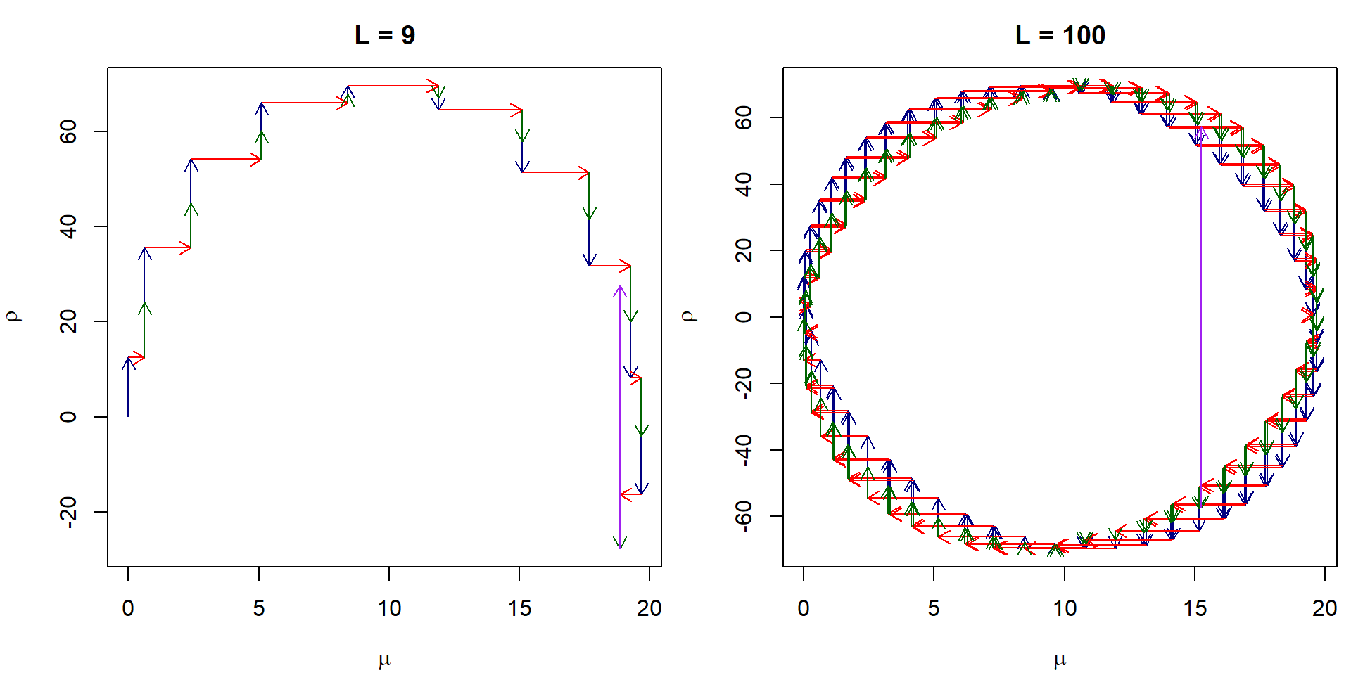 This is how the leapfrog integrator works if we start close to the
probability mass of the posterior, notice the change in the scale of the
individual steps:
This is how the leapfrog integrator works if we start close to the
probability mass of the posterior, notice the change in the scale of the
individual steps:
rho0 <- rnorm(1, sd = sqrt(sigmarho2))
L <- 10
par(mfrow = c(1,2), mar = c(4,4,2.5,0.5))
leapfrogs <- leapfrog_path_example(data, rho0 = rho0, mu0 = 10, L = L, eps = 0.05)
plot(leapfrogs$rho ~ leapfrogs$mu, type = "n",
     xlab = expression(mu), ylab = expression(rho), main = "L = 9",
     xlim = range(leapfrogs$mu), ylim = range(leapfrogs$rho, leapfrogs$rho1, leapfrogs$rho2))
arrows(x0 = leapfrogs$mu[1:L],
       y0 = leapfrogs$rho[1:L], y1 = leapfrogs$rho1[2:(L+1)], col = "navyblue", length = 0.1)
arrows(x0 = leapfrogs$mu[1:L], x1 = leapfrogs$mu[2:(L+1)],
       y0 = leapfrogs$rho1[2:(L+1)], col = "red", length = 0.1)
arrows(x0 = leapfrogs$mu[2:(L+1)],
       y0 = leapfrogs$rho1[2:(L+1)], y1 = leapfrogs$rho2[2:(L+1)], col = "darkgreen", length = 0.1)
arrows(x0 = leapfrogs$mu[(L+1)],
       y0 = leapfrogs$rho2[(L+1)], y1 = leapfrogs$rho[(L+1)], col = "purple", length = 0.1)

L <- 100
leapfrogs <- leapfrog_path_example(data, rho0 = rho0, mu0 = 10, L = L, eps = 0.05)
plot(leapfrogs$rho ~ leapfrogs$mu, type = "n",
     xlab = expression(mu), ylab = expression(rho), main = "L = 100",
     xlim = range(leapfrogs$mu), ylim = range(leapfrogs$rho, leapfrogs$rho1, leapfrogs$rho2))
arrows(x0 = leapfrogs$mu[1:L],
       y0 = leapfrogs$rho[1:L], y1 = leapfrogs$rho1[2:(L+1)], col = "navyblue", length = 0.1)
arrows(x0 = leapfrogs$mu[1:L], x1 = leapfrogs$mu[2:(L+1)],
       y0 = leapfrogs$rho1[2:(L+1)], col = "red", length = 0.1)
arrows(x0 = leapfrogs$mu[2:(L+1)],
       y0 = leapfrogs$rho1[2:(L+1)], y1 = leapfrogs$rho2[2:(L+1)], col = "darkgreen", length = 0.1)
arrows(x0 = leapfrogs$mu[(L+1)],
       y0 = leapfrogs$rho2[(L+1)], y1 = leapfrogs$rho[(L+1)], col = "purple", length = 0.1)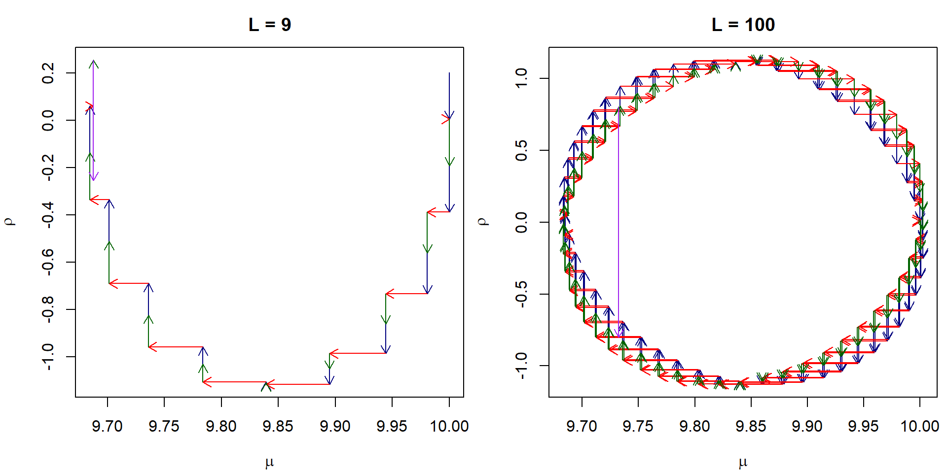
Now we implement the whole Hamiltonian Monte Carlo:
leapfrog_example <- function(data, rho0, mu0, L = 10, eps = 0.01, sigmarho2 = 1, sigma02 = 1, mumu = 5, sigmamu2 = 100){
  rho <- rho0
  mu <- mu0
  post_prec <- length(data)/sigma02 + 1/sigmamu2
  post_mean <- (sum(data) / sigma02 + mumu/sigmamu2)
  for(l in 1:L){
    rho <- rho1 <- rho + eps/2 * (post_mean - mu * post_prec)
    mu <- mu + eps * rho / sigmarho2
    rho <- rho2 <- rho + eps/2 * (post_mean - mu * post_prec)
  }
  # negate the momentum to get reversibility
  rho <- -rho
  return(list(rho = rho, mu = mu))
}

example_HamMC <- function(data, mu0, M, sigmarho2 = 1, sigma02 = 1, mumu = 5, sigmamu2 = 100, ...){
  mu <- accepted <- numeric(M)
  last <- mu0
  n <- length(data)
  ybar <- mean(data)
  loglast <- -n/2/sigma02*(last^2 - 2*last*ybar) - (last - mumu)^2/2/sigmamu2
  for(m in 1:M){
    rho0 <- rnorm(1, sd = sqrt(sigmarho2))
    logrho0 <- -rho0^2/2/sigmarho2
    proposal <- leapfrog_example(data, rho0 = rho0, mu0 = last,
                                 sigmarho2 = sigmarho2, sigma02 = sigma02,
                                 mumu = mumu, sigmamu2 = sigmamu2, ...)
    logmu <- -n/2/sigma02*(proposal$mu^2 - 2*proposal$mu*ybar) - (proposal$mu - mumu)^2/2/sigmamu2
    logrho <- -proposal$rho^2/2/sigmarho2
    prob <- min(1, exp(logmu + logrho - loglast - logrho0))
    accepted[m] <- rbinom(1, 1, prob)
    if(accepted[m]){
      last <- mu[m] <- unlist(proposal$mu)
      loglast <- logmu
    }else{
      mu[m] <- last
    }
  }

  return(list(mu = mu, accepted = accepted))
}
Let us sample only the first 100 steps to see that it is able to converge to the center of posterior:
mcmc1 <- example_HamMC(data, mu0 = 0, M = 100, L = 10, eps = 0.01)
mcmc2 <- example_HamMC(data, mu0 = 0, M = 100, L = 10, eps = 0.05)
# traceplots
par(mfrow = c(1,2), mar = c(4,4,2.5,0.5))
plot(mcmc1$mu, type = "l", main = "Epsilon = 0.01, L = 10", ylab = expression(mu))
plot(mcmc2$mu, type = "l", main = "Epsilon = 0.05, L = 10", ylab = expression(mu))
Now we sample the full chain of length 10000:
mcmc <- example_HamMC(data, mu0 = 10, M = 10000, L = 10, eps = 0.01)
summary(mcmc$mu)
## Min. 1st Qu. Median Mean 3rd Qu. Max.
## 9.325 9.740 9.836 9.836 9.932 10.304quantile(mcmc$mu, probs = c(0.025, 0.975))## 2.5% 97.5%
## 9.554128 10.114630par(mfrow = c(2,2), mar = c(4,4,3,0.5))
plot(mcmc$mu, type = "l", main = "Epsilon = 0.01, L = 10", ylab = expression(mu))
plot(ecdf(mcmc$mu), xlab = expression(mu), main = "Empirical CDF")
plot(density(mcmc$mu), xlab = expression(mu), main = "Kernel density estimator")
acf(mcmc$mu, main = "Autocorrelation function")
Stan and RStan
Install RStan library into your interface:
install.packages("rstan")library(rstan)If any troubles with the installation occur, please, visit the RStan Getting Started Github page.
The Stan User’s Guide contains a large number of implemented models, which you can use to understand its workflow. We will showcase its use on the AR(1)-GARCH(1) model, which is partially contained in Time-Series Models section.
Similarly as with JAGS, we need to supply input data and model definition. RStan distinguishes many different data types:
- data,
- transformed data,
- parameters,
- transformed parameters,
- model,
- generated quantities,
see Program Blocks section of the manual. See also the previous Statements section to understand all possible commands in RStan. The notation is very similar to R and JAGS but with couple of changes. Better to show on an example.
data(EuStockMarkets)
dax <- diff(log(EuStockMarkets[,1]))
dataAR1GARCH11 <- list(n = length(dax),
                       y = dax,
                       sigma1 = 1,
                       y0 = 0)
AR(1)-GARCH(1,1) model has the following implementation in RStan
(notice the change in the chunk type to stan instead of
r):
# data - input data not to be changed
data {
  int<lower=0> n;                         # type int/real needed!
  array[n] real y;                        # array for vectors, matrices, etc.
  real<lower=0> sigma1;                   # <lower=, upper=> restrictions of the domain
  real y0;                                # y[0] initial values for AR(1)
}

# parameters - primary model parameters
parameters {
  real a0;                                # a0 coefficient
  real a1;                                # a1 coefficient for AR(1)
  real<lower=0> alpha0;                   # alpha0 > 0 (no exp transformation)
  real<lower=0, upper=1> alpha1;          # alpha1 in (0,1) (transformation automatically)
  real<lower=0, upper=(1-alpha1)> beta1;  # beta1 in (0, 1-alpha1) (stationarity condition)
}

# auxiliary model parameters - transformation of data and parameters
transformed parameters {
  array[n] real mu;                       # means for data y
  array[n] real<lower=0> sigma;           # standard deviations for data y
  array[n] real eta;                      # residual terms
  real lalpha0;                           # transformed parameters
  real lalpha1;                           # by logarithm to real numbers
  real lbeta1;                            # as in ex-05a

  lalpha0 = log(alpha0);
  lalpha1 = log(alpha1);
  lbeta1 = log(beta1);

  mu[1] = a0 + a1 * y0;                   # initial mu
  eta[1] = y[1] - mu[1];
  sigma[1] = sigma1;                      # initial sigma

  for (t in 2:n) {
    mu[t] = a0 + a1 * y[t-1];
    eta[t] = y[t] - mu[t];
    sigma[t] = sqrt(alpha0 + alpha1 * pow(eta[t-1], 2) + beta1 * pow(sigma[t-1], 2));
  }
}

# model - describe, how the data are generated
model {
  ## Data generating process
  y ~ normal(mu, sigma); # increments the target probability log-density
  # target += normal_lupdf(y | mu, sigma) # manual equivalent increment to the target log-density

  ## Prior distributions
  a0 ~ normal(0, sqrt(3));
  a1 ~ normal(0, sqrt(3));
  lalpha0 ~ normal(-12.3, sqrt(5));
  lalpha1 ~ normal(-2, sqrt(5));
  lbeta1 ~ normal(-0.2, sqrt(5));
}
The model parameters are secretly transformed into a vector of parameters that are no longer restricted, which is required by the leapfrog integrator of Hamiltonian Monte Carlo. See the Constraint Transforms section in the manual for details on which functions are used.
In the list of continuous unbounded distributions we can find the parametrization of normal distribution (here mean and standard deviation). Notice also the following functions:
normal_lpdf- log-density,normal_lupdf- log-density without constant additive terms,normal_cdf- cumulative distribution function,normal_lcdf- log cumulative distribution function,normal_lccdf- log of complementary cumulative distribution function,normal_rng- generates random variable.
The chunk above defines model named AR1GARCH11, which is
then sampled by
pars <- c("a0", "a1", "alpha0", "alpha1", "beta1", "lalpha0", "lalpha1", "lbeta1")
# If AR1GARCH11 refers to the stan chunk above
mcmc <- stan(AR1GARCH11,
             data = dataAR1GARCH11,
             pars = pars,
             chains = 4, iter = 2000, warmup = floor(2000/2), thin = 1,
             seed = 123456789, init = 'random')

# # If AR1GARCH11 is a string containing model definition:
# mcmc <- stan(model_code = AR1GARCH11,
#              data = dataAR1GARCH11,
#              pars = pars,
#              chains = 4, iter = 2000, warmup = floor(2000/2), thin = 1,
#              see = 123456789, init = 'random')

plot(mcmc, pars = pars)
traceplot(mcmc, pars = pars)

# Continue in sampling
mcmc <- stan(fit = mcmc,
             data = dataAR1GARCH11,
             pars = pars,
             iter = 10000, verbose = F)
save(list = "mcmc", file = file.path(DATA, "mcmc_AR1GARCH11.RData"))
load(file.path(DATA, "mcmc_AR1GARCH11.RData"))Let’s examine the sampledchains.
class(mcmc)## [1] "stanfit"
## attr(,"package")
## [1] "rstan"print(mcmc)## Inference for Stan model: anon_model.
## 4 chains, each with iter=10000; warmup=5000; thin=1;
## post-warmup draws per chain=5000, total post-warmup draws=20000.
##
## mean se_mean sd 2.5% 25% 50% 75% 97.5% n_eff Rhat
## a0 0.00 0.00 0.00 0.00 0.00 0.00 0.00 0.00 22387 1
## a1 0.01 0.00 0.03 -0.04 -0.01 0.01 0.02 0.06 10618 1
## alpha0 0.00 0.00 0.00 0.00 0.00 0.00 0.00 0.00 7345 1
## alpha1 0.13 0.00 0.01 0.11 0.12 0.13 0.14 0.16 7252 1
## beta1 0.81 0.00 0.01 0.79 0.80 0.81 0.81 0.82 15167 1
## lalpha0 -11.94 0.00 0.14 -12.22 -12.02 -11.93 -11.84 -11.68 7092 1
## lalpha1 -2.03 0.00 0.09 -2.22 -2.10 -2.03 -1.97 -1.85 7258 1
## lbeta1 -0.22 0.00 0.01 -0.24 -0.22 -0.22 -0.21 -0.20 15191 1
## lp__ 7624.13 0.02 1.60 7620.17 7623.30 7624.46 7625.30 7626.24 6838 1
##
## Samples were drawn using NUTS(diag_e) at Mon Jan 5 15:03:41 2026.
## For each parameter, n_eff is a crude measure of effective sample size,
## and Rhat is the potential scale reduction factor on split chains (at
## convergence, Rhat=1).# summary(mcmc)
library(coda)
# convert into mcmc.list object from coda package --> we already know how to work with it
codamcmc <- As.mcmc.list(mcmc)
summary(codamcmc)##
## Iterations = 5001:10000
## Thinning interval = 1
## Number of chains = 4
## Sample size per chain = 5000
##
## 1. Empirical mean and standard deviation for each variable,
## plus standard error of the mean:
##
## Mean SD Naive SE Time-series SE
## a0 8.019e-04 2.041e-04 1.444e-06 1.354e-06
## a1 7.019e-03 2.568e-02 1.816e-04 2.487e-04
## alpha0 6.618e-06 9.057e-07 6.405e-09 1.073e-08
## alpha1 1.315e-01 1.225e-02 8.663e-05 1.411e-04
## beta1 8.054e-01 8.300e-03 5.869e-05 6.647e-05
## lalpha0 -1.194e+01 1.382e-01 9.772e-04 1.664e-03
## lalpha1 -2.033e+00 9.338e-02 6.603e-04 1.073e-03
## lbeta1 -2.165e-01 1.030e-02 7.286e-05 8.244e-05
## lp__ 7.624e+03 1.596e+00 1.128e-02 1.890e-02
##
## 2. Quantiles for each variable:
##
## 2.5% 25% 50% 75% 97.5%
## a0 4.000e-04 6.644e-04 8.032e-04 9.379e-04 1.203e-03
## a1 -4.297e-02 -1.024e-02 7.113e-03 2.430e-02 5.732e-02
## alpha0 4.923e-06 5.999e-06 6.583e-06 7.216e-06 8.474e-06
## alpha1 1.088e-01 1.230e-01 1.312e-01 1.397e-01 1.567e-01
## beta1 7.893e-01 7.997e-01 8.053e-01 8.110e-01 8.219e-01
## lalpha0 -1.222e+01 -1.202e+01 -1.193e+01 -1.184e+01 -1.168e+01
## lalpha1 -2.218e+00 -2.096e+00 -2.031e+00 -1.968e+00 -1.853e+00
## lbeta1 -2.366e-01 -2.236e-01 -2.166e-01 -2.095e-01 -1.962e-01
## lp__ 7.620e+03 7.623e+03 7.624e+03 7.625e+03 7.626e+03Plot depicting the posterior distribution of the model parameters. Maybe better to plot each separately due to different scales.
par(mar = c(4,4,2,0.5))
plot(mcmc)
Traceplots of the model parameters:
par(mar = c(4,4,2,0.5))
rstan::traceplot(mcmc)
Or ggplot versions of the plots:
library(ggplot2)
stan_dens(mcmc)
Autocorrelation function:
stan_ac(mcmc)
There are some diagnostic plots available as well:
stan_diag(mcmc)