Building Cox models for censored data (constant covariates)
Jan Vávra
Exercise 7 (17th December 2019)
Theory - the Cox model with time-invariant covariates
We observe \(n\) independent triplets \((X_i, \delta_i, \mathbf{Z}_i), i = 1, \ldots, n\), where
- \(X_i = \min \{T_i, C_i\}\) is censored failure time,
- \(\delta_i = \mathbb{I}_{(T_i \leq C_i)}\) is failure indicator,
- \(\mathbf{Z}_i\) is a vector of covariates.
The Cox model is used to estimate the effect of covariates \(\mathbf{Z}_i\) on continuous (but arbitrary) distribution of failure times \(T_i\) and to test its significance.
In this exercise we will deal with covariates constant in time.
We suppose that the hazard function \(\lambda\) of failure time distribution (assumed to be continuous) given covariates \(T|\mathbf{Z}\) is of the form: \[\lambda(t| \mathbf{Z}) = \lambda_0(t) \exp \left\{ \boldsymbol{\beta}^{\mathsf{T}} \mathbf{Z} \right\},\] where:
- \(\lambda_0(t)\) is the baseline hazard function,
- \(\boldsymbol{\beta} \in \mathbb{R}^p\) is unknown vector of regression coefficients.
Notes:
- See the difference in \(\lambda_0(t)\) (no required shape) compared to \(\lambda_0\) from Exercise 1.
- No intercept included in \(\mathbf{Z}_i\), it is covered by \(\lambda_0(t)\).
- The Cox “proportional hazard” model (under constant covariates) refers to the property of ratio of hazard functions with different covariates:
\[\dfrac{\lambda(t| \mathbf{Z}_1)}{\lambda(t| \mathbf{Z}_2)} = \dfrac{\lambda_0(t)}{\lambda_0(t)} \cdot \dfrac{\exp \left\{ \boldsymbol{\beta}^{\mathsf{T}} \mathbf{Z}_1 \right\}}{\exp \left\{ \boldsymbol{\beta}^{\mathsf{T}} \mathbf{Z}_2 \right\}} = \exp \left\{ \boldsymbol{\beta}^{\mathsf{T}} (\mathbf{Z}_1 - \mathbf{Z}_2) \right\} \quad \text{is constant in time } t.\] Interpretation of \(\beta_j\) coefficient can be derived in the usual way: \[\exp \beta_j = \dfrac{\lambda(t| \mathbf{Z} + \mathbf{e}_j)}{\lambda(t| \mathbf{Z})}.\]
In the case of constant regressors we can express the Cox model in the terms of survival functions:
- \(\Lambda_0(t) = \int \limits_0^{t} \lambda_0(s) \, \mathrm{d} s\) is the cumulative baseline hazard,
- \(S_0(t) = \exp \left\{- \Lambda_0(t) \right\}\) is the baseline survival function,
- general survival function \(S(t|\mathbf{Z})\) is of the form: \[S(t|\mathbf{Z}) = \left[S_0(t)\right]^{\exp \boldsymbol{\beta}^{\mathsf{T}} \mathbf{Z} }.\]
Model is estimated by partial likelihood method that shares properties with classical maximum likelihood method. We can perform tests for:
- single covariates \(\beta_j\): \[\sqrt{n} \dfrac{ \widehat{\beta}_j - \beta_j}{\sqrt{\left(\mathcal{I}_{n}^{-1}\right)_{jj}(\widehat{\boldsymbol{\beta}}, \tau)} } \overset{\mathcal{D}}{\longrightarrow} \mathsf{N}(0,1),\]
- linear combinations of \(\boldsymbol{\beta}\): \[\sqrt{n} \dfrac{ \mathbf{c}^{\mathsf{T}} \widehat{\boldsymbol{\beta}} - \mathbf{c}^{\mathsf{T}} \boldsymbol{\beta} }{\sqrt{\boldsymbol{c}^{\mathsf{T}} \mathcal{I}_{n}^{-1}(\widehat{\boldsymbol{\beta}}, \tau) \boldsymbol{c}} } \overset{\mathcal{D}}{\longrightarrow} \mathsf{N}(0,1),\]
- submodel testing (\(\ell_M (\widehat{\boldsymbol{\beta}})\), \(\ell_S (\widetilde{\boldsymbol{\beta}})\) are maximized partial log-likehoods of model and submodel): \[2 \left( \ell_M (\widehat{\boldsymbol{\beta}}) - \ell_S (\widetilde{\boldsymbol{\beta}}) \right) \overset{\mathcal{D}}{\longrightarrow} \chi_m^2, \quad \text{where } m \text{ is the difference in number of parameters.}\]
We can use the Breslow estimator of cumulative baseline hazard function \[ \widehat{\Lambda}_0(t) = \int \limits_{0}^{t} \dfrac{ \, \mathrm{d} \overline{N}(s)}{\sum \limits_{i=1}^n Y_i (s) \exp \left\{ \widehat{\boldsymbol{\beta}}^{\mathsf{T}} \mathbf{Z}_i \right\}} \] to obtain an estimate of general survival function \[ \widehat{S}(t| \mathbf{Z}) = \exp \left\{ - \widehat{\Lambda}(t| \mathbf{Z})\right\} = \exp \left\{ - \widehat{\Lambda}_0(t) \exp \left\{ \widehat{\boldsymbol{\beta}}^{\mathsf{T}} \mathbf{Z} \right\} \right\}. \]
Obtaining and investigating the dataset
We will work with the dataset pbc contained in the survival library, see Exercise 1 or help(pbc) for description.
library(survival)
data(pbc)
variables <- c("id", "time", "status", "trt", "sex", "edema", "bili", "albumin", "platelet")
data <- pbc[, variables]
We will work with the following variables:
| Var. name | Description |
|---|---|
| id | case number |
| status | status at the end of follow-up: 0 = censored, 1 = transplanted, 2 = dead |
| time | number of days of follow-up |
| trt | treatment: 1 = D-penicillamin, 2 = placebo, NA = not randomised |
| sex | sex m/f |
| edema | 0 = no edema, 0.5 = untreated or successfully treated, 1 = edema despite diuretic therapy |
| bili | serum bilirubin (mg/dl) |
| albumin | serum albumin (g/dl) |
| platelet | platelet count |
Here are initial rows of the dataset:
head(data)## id time status trt sex edema bili albumin platelet
## 1 1 400 2 1 f 1.0 14.5 2.60 190
## 2 2 4500 0 1 f 0.0 1.1 4.14 221
## 3 3 1012 2 1 m 0.5 1.4 3.48 151
## 4 4 1925 2 1 f 0.5 1.8 2.54 183
## 5 5 1504 1 2 f 0.0 3.4 3.53 136
## 6 6 2503 2 2 f 0.0 0.8 3.98 NAWe are interested in modelling survival time in untransplanted patients. Patients who had liver transplant will be censored at the moment the transplant was done. Therefore, similarly as in Exercise 1 define \(\delta\) indicator as
data$delta = (data$status == 2)Explorative analysis
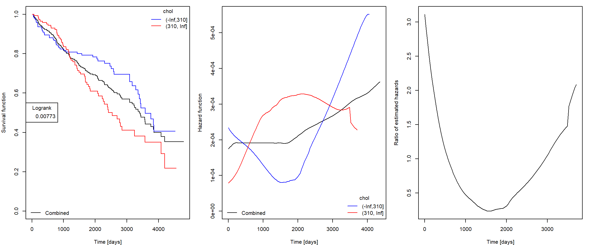
First, we will start with explorative analysis using methods we already know - non-parametric estimation of survival function (Kaplan-Meier) and logrank test for comparing two (possibly more) different groups.
- Choose one binary and one continuous variable.
- Cut continuous variable into two groups (by value “near” median).
- Take binary variable and the created one and perform two-sample analysis.
- Plot survival curves and calculate logrank tests.
- Notice whether the chosen variables look associated with survival.
- Plot smoothed estimate of hazard function and try to justify the proportionality assumption of the Cox model.
An illustration of possible output (try to optimize your code so that it can be easily used for several variables):
Estimating Cox model
The function to fit the Cox proportional hazards model is called coxph. It’s syntax is [example]
fit <- coxph(Surv(time,delta)~log(age)+chol+hepato,data=pbc)See help(coxph) for additional parameters such as weights (in case of repeated observations), na.action (missing-data filter function), ties (methods for tie handling), …
You can use function summary to view \(\boldsymbol{\beta}\) coefficient estimates (including exponentiated versions):
summary(fit)## Call:
## coxph(formula = Surv(time, delta) ~ log(age) + chol + hepato,
## data = pbc)
##
## n= 284, number of events= 114
## (134 observations deleted due to missingness)
##
## coef exp(coef) se(coef) z Pr(>|z|)
## log(age) 2.406e+00 1.109e+01 5.231e-01 4.599 4.24e-06 ***
## chol 1.152e-03 1.001e+00 3.134e-04 3.675 0.000238 ***
## hepato 8.941e-01 2.445e+00 2.051e-01 4.358 1.31e-05 ***
## ---
## Signif. codes: 0 '***' 0.001 '**' 0.01 '*' 0.05 '.' 0.1 ' ' 1
##
## exp(coef) exp(-coef) lower .95 upper .95
## log(age) 11.087 0.09019 3.977 30.910
## chol 1.001 0.99885 1.001 1.002
## hepato 2.445 0.40899 1.636 3.655
##
## Concordance= 0.714 (se = 0.023 )
## Likelihood ratio test= 56.08 on 3 df, p=4e-12
## Wald test = 53.26 on 3 df, p=2e-11
## Score (logrank) test = 57.36 on 3 df, p=2e-12Survival probabilities calculation
In our example consider patient of age 50 with hepatomegaly and serum cholesterol 300 mg/dl.
There exists predict.coxph function that seems to be useful for calculating survival probabilities, however, I strongly recommend not to use it! See Details of predict.coxph: reference values for baseline are means of covariates.
Estimator of baseline cumulative hazard \(\widehat{\Lambda}_0(t)\) can be obtained using function basehaz with option centered = F. General cumulative hazard function estimator can be obtained by combination of basehaz and corresponding exponentiated linear predictor. Survival function estimator can be obtained using \(S = \exp \left\{ - \Lambda\right\}\) transformation:
L0 <- basehaz(fit, centered = F)
# Manual calculation of exp(linear predictor)
patient_LinPred <- sum(c(log(50), 300, 1)*fit$coefficients)
patient_Lambda <- L0$hazard * exp(patient_LinPred)

par(mfrow = c(1,2), mar = c(4,4,1,1))
plot(patient_Lambda~L0$time, type = "s", col = "skyblue", xlab = "Time [days]", ylab = "Cumulative hazard")

plot(exp(-patient_Lambda)~L0$time, type = "s", col = "skyblue", ylim = c(0,1),
     xlab = "Time [days]", ylab = "Survival probability")
More practical way is to supply newdata to survfit function applied to fit object (output of coxph function):
newdata <- data.frame(age = 50, chol = 300, hepato = 1)
fitnew <- survfit(fit, newdata = newdata, conf.type = "plain")

par(mfrow = c(1,2), mar = c(4,4,1,1))
plot(fitnew, fun = "cumhaz", xlab = "Time [Days]", ylab = "Cumulative hazard", col = "skyblue", conf.int = F)
plot(fitnew, xlab = "Time [Days]", ylab = "Survival probability", col = "skyblue")
You can use libraries ggplot2 and survminer to obtain visually nice plots:
library(survminer)
library(ggplot2)

newdata <- with(pbc, data.frame(age =    c( 50,  50,        50),
                                chol =   c(300, 300,       300),
                                hepato = c(  1,   0, 0.5176056)))
fitnew <- survfit(fit, newdata = newdata, conf.type = "plain")

ggsurvplot(fitnew, data = newdata,
           conf.int = TRUE, censor= FALSE,
           legend.labs=c("Patient 1", "Patient 2", "Patient 3"),
           ggtheme = theme_minimal())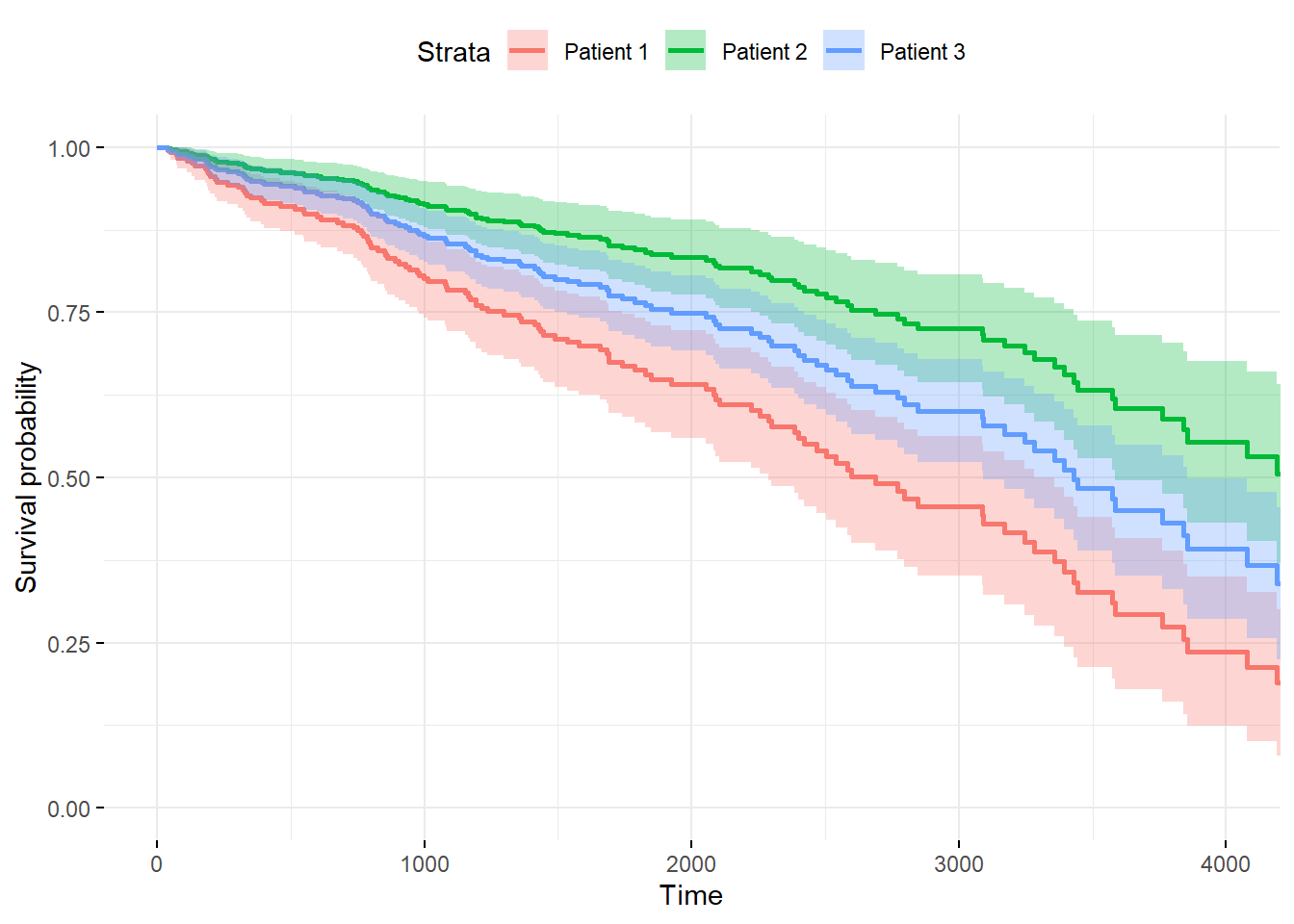
Investigating treatment and bilirubin by Cox model
- Fit the Cox proportional hazards model with treatment as the single covariate.
- Interpret the estimated parameter and its confidence interval.
- Test the hypothesis that treatment has no effect on survival of PBC patients.
- Plot estimated survival functions for both groups based on the Cox model and compare them with Kaplan-Meier estimators of the corresponding two samples.
- Compare the results with the logrank test.
- Fit the Cox proportional hazards model with grouped bilirubin (four groups defined by sample quartiles) as the single covariate.
- Interpret the estimated parameters.
- Test the hypothesis that bilirubin does not affect survival of PBC patients.
- Plot estimated survival functions of these four groups based on the Cox model and compare them with Kaplan-Meier estimators of the corresponding four samples.
- Consider a suitable transformation for continuous bilirubin (see next task).
Cox model with multiple covariates
The logic of specifying the model formula is the same as with functions lm or glm. Printing the results and performing tests of hypotheses for model building is also very similar to other regression functions in R:
summary(fit)
anova(fit)
anova(fit1,fit2)
drop1(fit,test="Chisq")
add1(fit, scope = "bili:trt", test = "Chisq")
The parameter estimation is based on the maximum partial likelihood method but the asymptotic properties, tests etc. are all the same as with ordinary likelihood methods. In particular, a submodel is tested against a wider model by likelihood ratio tests performed by functions anova or drop1. The difference of log-partial-likelihoods multiplied by 2 has asymptotically \(\chi^2_m\) distribution if the submodel is true, where \(m\) is the difference in the number of parameters. The tests shown in the parameter table of summary function are Wald tests for zero values of the individual parameters.
- Build the Cox proportional hazards model for survival of PBC patients.
- Include treatment in the model; consider other variables of interest as additional covariates.
- Continuous variables can be included in the linear form, or after transformation, or in the grouped form.
- Do not include interactions.
- Keep only the covariates that have a significant effect on survival (except treatment).
- Interpret the effect of treatment as well as of other covariates that have been kept in the final model.
- Show confidence intervals for their effects.
- Test their effects on survival of PBC patients.
- Plot estimated survival function depending on the value of treatment (fix reasonably the values of other remaining covariates).
- Compare your final Cox model with your final model from Exercise 1.
- What is the main difference in the model definition and structure?
- Compare the results regarding significance of treatment.
- Is the subset of significant covariates the same as before? Are the chosen parametrizations of covariates the same?
- Any other interesting comparisons?
- Deadline for report: next exercise class 6th January