Multiple regression model - numeric covariates
Jan Vávra
Exercise 4
Download this R markdown as: R, Rmd.
Outline of the lab session
- Multiple regression model for the continuous response vector with continuous regressors
- K-variate parametrizations of a numeric covariate
Loading the data and libraries
The dataset mtcars (available under the standard R
installation) will be used for the purposes of this lab session. Some
insight about the data can be taken from the help session (command
?mtcars) or from some outputs provided below.
library(colorspace)
head(mtcars)
## mpg cyl disp hp drat wt qsec vs am gear carb
## Mazda RX4 21.0 6 160 110 3.90 2.620 16.46 0 1 4 4
## Mazda RX4 Wag 21.0 6 160 110 3.90 2.875 17.02 0 1 4 4
## Datsun 710 22.8 4 108 93 3.85 2.320 18.61 1 1 4 1
## Hornet 4 Drive 21.4 6 258 110 3.08 3.215 19.44 1 0 3 1
## Hornet Sportabout 18.7 8 360 175 3.15 3.440 17.02 0 0 3 2
## Valiant 18.1 6 225 105 2.76 3.460 20.22 1 0 3 1str(mtcars)## 'data.frame': 32 obs. of 11 variables:
## $ mpg : num 21 21 22.8 21.4 18.7 18.1 14.3 24.4 22.8 19.2 ...
## $ cyl : num 6 6 4 6 8 6 8 4 4 6 ...
## $ disp: num 160 160 108 258 360 ...
## $ hp : num 110 110 93 110 175 105 245 62 95 123 ...
## $ drat: num 3.9 3.9 3.85 3.08 3.15 2.76 3.21 3.69 3.92 3.92 ...
## $ wt : num 2.62 2.88 2.32 3.21 3.44 ...
## $ qsec: num 16.5 17 18.6 19.4 17 ...
## $ vs : num 0 0 1 1 0 1 0 1 1 1 ...
## $ am : num 1 1 1 0 0 0 0 0 0 0 ...
## $ gear: num 4 4 4 3 3 3 3 4 4 4 ...
## $ carb: num 4 4 1 1 2 1 4 2 2 4 ...summary(mtcars)## mpg cyl disp hp drat wt
## Min. :10.40 Min. :4.000 Min. : 71.1 Min. : 52.0 Min. :2.760 Min. :1.513
## 1st Qu.:15.43 1st Qu.:4.000 1st Qu.:120.8 1st Qu.: 96.5 1st Qu.:3.080 1st Qu.:2.581
## Median :19.20 Median :6.000 Median :196.3 Median :123.0 Median :3.695 Median :3.325
## Mean :20.09 Mean :6.188 Mean :230.7 Mean :146.7 Mean :3.597 Mean :3.217
## 3rd Qu.:22.80 3rd Qu.:8.000 3rd Qu.:326.0 3rd Qu.:180.0 3rd Qu.:3.920 3rd Qu.:3.610
## Max. :33.90 Max. :8.000 Max. :472.0 Max. :335.0 Max. :4.930 Max. :5.424
## qsec vs am gear carb
## Min. :14.50 Min. :0.0000 Min. :0.0000 Min. :3.000 Min. :1.000
## 1st Qu.:16.89 1st Qu.:0.0000 1st Qu.:0.0000 1st Qu.:3.000 1st Qu.:2.000
## Median :17.71 Median :0.0000 Median :0.0000 Median :4.000 Median :2.000
## Mean :17.85 Mean :0.4375 Mean :0.4062 Mean :3.688 Mean :2.812
## 3rd Qu.:18.90 3rd Qu.:1.0000 3rd Qu.:1.0000 3rd Qu.:4.000 3rd Qu.:4.000
## Max. :22.90 Max. :1.0000 Max. :1.0000 Max. :5.000 Max. :8.0001. Multiple linear regression model
For simplicity, we will only consider three explanatory (continuous)
variables from the whole mtcars dataset, i.e. \(\boldsymbol{x} \in \mathbb{R}^3\). Any
generalization for general \(\boldsymbol{X}
\in \mathbb{R}^p\) for some \(p \in
\mathbb{N}\) is straightforward. In particular, the (continuous)
dependent variable \(Y \in \mathbb{R}\)
is the car consumption (variable in the dataset denoted as
mpg – miles per gallon) and three independent variables
will be the car’s displacement (disp), horse powers
(hp), and the rear axle ratio information
(drat).
Three simple scatterplots showing the dependent variable \(Y\) against one independent variable (based on the random sample \(\{(Y_i, \boldsymbol{X}_i^\top)^\top;~i = 1, \dots, 32\}\)) are shown below. Only a limited information about the whole multivariate structure of the underlying data can be, howver, taken from the series of two-dimensional scatterplots.
par(mfrow = c(1,3), mar = c(4,4,0.5,0.5))
plot(mpg ~ disp, data = mtcars, pch = 22, cex = 0.8, bg = "lightblue",
     ylab = "Miles per gallon", xlab = "Displacement [cubic inches]")
lines(lowess(mtcars$mpg ~ mtcars$disp), col = "red", lwd = 2)
plot(mpg ~ hp, data = mtcars, pch = 22, cex = 0.8, bg = "lightblue",
     ylab = "", xlab = "Horse Power")
lines(lowess(mtcars$mpg ~ mtcars$hp), col = "red", lwd = 2)
plot(mpg ~ drat, data = mtcars, pch = 22, cex = 0.8, bg = "lightblue",
     ylab = "", xlab = "Rear axle ratio")
lines(lowess(mtcars$mpg ~ mtcars$drat), col = "red", lwd = 2)
The red curves are non-parametric estimates of the conditional mean—these estimates offer a useful insight that the dependence of the consumptions is very likely negative (regressive) wrt. the displacement and horsepower while it seems to positive (progressive) for the rear axle ratio.
A simple multiple regression model of the form \[ Y = \beta_1 + \beta_2 \mathtt{disp} + \beta_3\mathtt{hp} + \beta_4 \mathtt{drat} + \varepsilon \] or mathematically (the model for the empirical data, for \(i = 1, \dots, 32\)) \[ Y_i = \boldsymbol{X}_i^\top\boldsymbol{\beta} + \varepsilon_i \] where \(\boldsymbol{X} = (1, \mathtt{disp}, \mathtt{hp}, \mathtt{drat})^\top\) and \(\boldsymbol{\beta} \in \mathbb{R}^4\) will be considered. In the R software, the model can be fitted using the following R code:
fit1 <- lm(mpg ~ disp + hp + drat, data = mtcars)
print(fit1)
##
## Call:
## lm(formula = mpg ~ disp + hp + drat, data = mtcars)
##
## Coefficients:
## (Intercept) disp hp drat
## 19.34429 -0.01923 -0.03123 2.71498The information in the output above gives values for four estimated parameters – elements of the parameter vector \(\boldsymbol{\beta} \in \mathbb{R}^4\). The estimated parameters are not the same as estimated three independent simple linear regression model. Compare the output above with the following outputs:
fit_disp <- lm(mpg ~ disp, data = mtcars)
fit_hp <- lm(mpg ~ hp, data = mtcars)
fit_drat <- lm(mpg ~ drat, data = mtcars)

print(fit_disp)
##
## Call:
## lm(formula = mpg ~ disp, data = mtcars)
##
## Coefficients:
## (Intercept) disp
## 29.59985 -0.04122print(fit_hp)##
## Call:
## lm(formula = mpg ~ hp, data = mtcars)
##
## Coefficients:
## (Intercept) hp
## 30.09886 -0.06823print(fit_drat)##
## Call:
## lm(formula = mpg ~ drat, data = mtcars)
##
## Coefficients:
## (Intercept) drat
## -7.525 7.678Indeed, while the signs of the estimated parameters correspond, the magnitudes are substantially different. The ordinary regressions can be directly plotted into the corresponding scatterplots:
par(mfrow = c(1,3), mar = c(4,4,0.5,0.5))
plot(mpg ~ disp, data = mtcars, pch = 22, cex = 0.8, bg = "lightblue", ylab = "Miles per gallon", xlab = "Displacement [cubic inches]")
lines(lowess(mtcars$mpg ~ mtcars$disp), col = "red", lwd = 2)
abline(fit_disp, col = "blue")
plot(mpg ~ hp, data = mtcars, pch = 22, cex = 0.8, bg = "lightblue", ylab = "", xlab = "Horse Power")
lines(lowess(mtcars$mpg ~ mtcars$hp), col = "red", lwd = 2)
abline(fit_hp, col = "blue")
plot(mpg ~ drat, data = mtcars, pch = 22, cex = 0.8, bg = "lightblue", ylab = "", xlab = "Rear axle ratio")
lines(lowess(mtcars$mpg ~ mtcars$drat), col = "red", lwd = 2)
abline(fit_drat, col = "blue")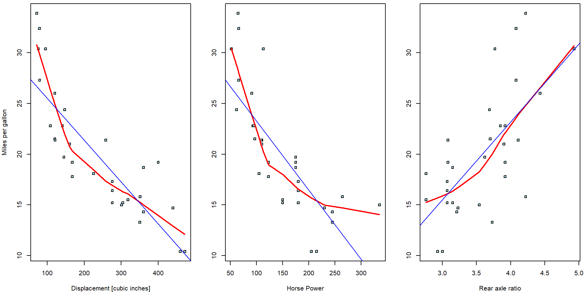
However, the multiple regression model does not estimate a line but a
three dimensional subspace. For instance, the intercept value \(\widehat{\beta}_0 = 29.6\) from the simple
regression model fit_disp stands for the expected driven
miles per one gallon if the displacement of the engine is equal to zero
cubic inches (i.e., an unrealistic scenario).
Nevertheless, the intercept estimate \(\widehat{\beta}_0 = 19.34\) stands for the expected driven miles per one gallon but if all three regressors – the information about the displacement, the horse powers, and, also, the rear to axel ratio – are all equal to zero. Therefore, to draw simple line for two-dimensional scatterplot, it is needed to pre-select some reasonable information (realistic case) for all other covariates in the model.
For instance, consider the multiple model from above and, in particular, the scatterplot of the consumption against the displacement. Various regression lines can be considered:
par(mfrow = c(1,1), mar = c(4,4,0.5,0.5))
plot(mpg ~ disp, data = mtcars, pch = 22, cex = 0.8, bg = "lightblue",
     xlab = "Displacement [cubic inches]", ylab = "Miles per gallon")

xGrid <- seq(min(mtcars$disp), max(mtcars$disp, 100))
mCoeff <- fit1$coeff

yMeanMean <- mCoeff[1] + mCoeff[2] * xGrid + mCoeff[3] * mean(mtcars$hp) + mCoeff[4] * mean(mtcars$drat)
lines(yMeanMean ~ xGrid, col = "red", lwd = 2)

yMinMin <- mCoeff[1] + mCoeff[2] * xGrid + mCoeff[3] * min(mtcars$hp) + mCoeff[4] * min(mtcars$drat)
yMaxMax<- mCoeff[1] + mCoeff[2] * xGrid + mCoeff[3] * max(mtcars$hp) + mCoeff[4] * max(mtcars$drat)
lines(yMinMin ~ xGrid, col = "blue", lwd = 2, lty = 2)
lines(yMaxMax ~ xGrid, col = "darkgreen", lwd = 2, lty = 2)

legend("topright",
       legend = c("Average HP & average rear axle ratio",
                  "Min HP & min rear axle ratio",
                  "Max HP & max rear axle ratio"),
       col =c("red", "blue", "darkgreen"), lwd = c(3,3,3), lty = c(1,2,2))
Individual work
- The whole set of different regression lines can be plotted depending on particular choices for the remaining covariates that are not used in the scatterplot (in this case, the information about the horse powers and the rear axle ratio).
- For all three considered covariates draw a separate scatterplot with a set of regression lines that will reasonably explain the underlying dependence of the car consumption.
- In practical applications, it is reasonable to use the exploratory analysis to pre-select some reasonable values for the covariates that are used in the model formula, the relationship of the dependent covariate is not directly illustrated in the plot. For instance, one can use a series of nice curves for the estimated deciles of, let’s say the horse power, while always using the median value of the rear axle ratio.
2. Computations behind lm()
Consider the matrix notation of our problem \[ \mathbf{Y} = \begin{pmatrix} Y_1 \\ Y_2 \\ \vdots \\ Y_n \end{pmatrix} = \begin{pmatrix} \mathbf{X_1}^\top \\ \mathbf{X_2}^\top \\ \vdots \\\mathbf{X_n}^\top \end{pmatrix} \begin{pmatrix} \beta_1 \\ \beta_2 \\ \vdots \\ \beta_p \end{pmatrix} + \begin{pmatrix} \varepsilon_1 \\ \varepsilon_2 \\ \vdots \\ \varepsilon_n \end{pmatrix} = \mathbb{X} \boldsymbol{\beta} + \boldsymbol{\varepsilon}. \] Then, the sum of squares to be minimized could be written as \[ \mathsf{SS}(\boldsymbol{\beta}) = \sum\limits_{i=1}^n \left(Y_i - \mathbf{X}_i^\top \boldsymbol{\beta}\right)^2 = \left(\mathbf{Y} - \mathbb{X} \boldsymbol{\beta}\right)^\top \left(\mathbf{Y} - \mathbb{X} \boldsymbol{\beta}\right) = \mathbf{Y}^\top \mathbf{Y} - 2\mathbf{Y}^\top \mathbb{X} \boldsymbol{\beta} + \boldsymbol{\beta}^\top \mathbb{X}^\top \mathbb{X} \boldsymbol{\beta} . \] Since the derivatives are \[ \frac{\partial \mathsf{SS}(\boldsymbol{\beta})}{\partial \boldsymbol{\beta}} = 2 \mathbb{X}^\top \mathbb{X} \boldsymbol{\beta} - 2 \mathbb{X}^\top \mathbf{Y}, \qquad \frac{\partial^2 \mathsf{SS}(\boldsymbol{\beta})}{\partial \boldsymbol{\beta}\partial \boldsymbol{\beta}^\top} = 2 \mathbb{X}^\top \mathbb{X} \geq 0, \] the solution to the minimization problem can be found as a solution of \(\mathbb{X}^\top \mathbb{X} \boldsymbol{\beta} = \mathbb{X}^\top \mathbf{Y}\). In particular, \[ \widehat{\boldsymbol{\beta}} = \arg\min \mathsf{SS}(\boldsymbol{\beta}) = \left(\mathbb{X}^\top \mathbb{X}\right)^{-1} \mathbb{X}^\top \mathbf{Y}, \] when the inverse matrix exists (under full-rank model – all columns of \(\mathbb{X}\) linearly independent). In R we would compute it as follows:
X <- model.matrix(~ disp + hp + drat, data = mtcars)
dim(X)
## [1] 32 4head(X)## (Intercept) disp hp drat
## Mazda RX4 1 160 110 3.90
## Mazda RX4 Wag 1 160 110 3.90
## Datsun 710 1 108 93 3.85
## Hornet 4 Drive 1 258 110 3.08
## Hornet Sportabout 1 360 175 3.15
## Valiant 1 225 105 2.76XtX <- t(X) %*% X
XtY <- t(X) %*% mtcars$mpg
betahat <- solve(XtX, XtY)[,1]
all.equal(betahat, fit1$coefficients)## [1] TRUEThe vector of observed response values \(\mathbf{Y}\) now decomposes into a sum of two vectors \[ \mathbf{Y} = \widehat{\mathbf{Y}} + \left(\mathbf{Y} -\widehat{\mathbf{Y}}\right) = \mathbb{X} \widehat{\boldsymbol{\beta}} + \left(\mathbf{Y} -\mathbb{X} \widehat{\boldsymbol{\beta}}\right) = \underbrace{\mathbb{X}\left(\mathbb{X}^\top \mathbb{X}\right)^{-1} \mathbb{X}^\top}_{\mathbb{H}} \mathbf{Y} + \underbrace{\left(\mathbb{I}_n - \mathbb{X}\left(\mathbb{X}^\top \mathbb{X}\right)^{-1} \mathbb{X}^\top \right)}_{\mathbb{M}}\mathbf{Y}. \] The fitted values \(\widehat{\mathbf{Y}} = \mathbb{X} \widehat{\boldsymbol{\beta}} = \mathbb{H} \mathbf{Y}\) can be viewed as a projection of \(\mathbb{Y}\) into a subspace of \(\mathbb{R}^n\) generated by columns of \(\mathbb{X}\) – the regression space. The residuals \(\mathbf{U} = \mathbf{Y} - \widehat{\mathbf{Y}} = \mathbb{M} \mathbf{Y}\) can be viewed as a projection of \(\mathbb{Y}\) into the residual space orthogonal to the regression space. It is clear that for any \(\mathbf{Y}\in\mathbb{R}^n\) we have \[ \mathbf{U}^\top \widehat{\mathbf{Y}} = \mathbf{Y}^\top \mathbb{MH} \mathbf{Y} = \mathbf{Y}^\top \left[\mathbb{H} - \mathbb{X}\left(\mathbb{X}^\top \mathbb{X}\right)^{-1} \mathbb{X}^\top \mathbb{X}\left(\mathbb{X}^\top \mathbb{X}\right)^{-1} \mathbb{X}^\top \right] \mathbf{Y} = \mathbf{Y}^\top \left[\mathbb{H} - \mathbb{H} \right] \mathbf{Y} = 0. \]
Yhat <- X %*% betahat
all.equal(c(Yhat), unname(fitted(fit1)))
## [1] TRUEUres <- mtcars$mpg - Yhat
all.equal(c(Ures), unname(residuals(fit1)))## [1] TRUEsum(Yhat * Ures) # numerically orthogonal## [1] 4.790668e-12H <- X %*% solve(XtX) %*% t(X)
H[1:6, 1:6]## Mazda RX4 Mazda RX4 Wag Datsun 710 Hornet 4 Drive Hornet Sportabout Valiant
## Mazda RX4 0.04481605 0.04481605 0.046469903 0.02450713 0.015416659 0.01754638
## Mazda RX4 Wag 0.04481605 0.04481605 0.046469903 0.02450713 0.015416659 0.01754638
## Datsun 710 0.04646990 0.04646990 0.066552408 0.03375973 -0.002552776 0.05555439
## Hornet 4 Drive 0.02450713 0.02450713 0.033759734 0.10095654 0.062586688 0.12518346
## Hornet Sportabout 0.01541666 0.01541666 -0.002552776 0.06258669 0.081040947 0.04700280
## Valiant 0.01754638 0.01754638 0.055554394 0.12518346 0.047002800 0.20138324M <- diag(dim(H)[1]) - H
sum(abs(H %*% M)) # orthogonal to each other## [1] 5.374134e-13dim(H) # projection from R^n to regression subspace of R^n## [1] 32 32# lm() computation through QR decomposition
Q <- qr.Q(fit1[["qr"]]) # Q matrix (orthogonal columns)
all.equal(unname(H), Q %*% t(Q))## [1] TRUEall.equal(H %*% mtcars$mpg, Yhat)## [1] TRUEall.equal(M %*% mtcars$mpg, Ures)## [1] TRUEAs by-product, the vector of residuals is orthogonal to any column of matrix \(\mathbb{X}\): \[ \mathbb{X}^\top \mathbf{U} = \mathbb{X}^\top \mathbb{M} \mathbf{Y} = \left[\mathbb{X}^\top - \mathbb{X}^\top \mathbb{X} \left(\mathbb{X}^\top \mathbb{X}\right)^{-1}\mathbb{X}^\top \right] \mathbf{Y} = \mathbf{0}. \] Especially, when the vector of all ones \(\mathbf{1}\) is a column of \(\mathbb{X}\), also the sum (and subsequently the mean) of residuals \(\mathbf{1}^\top \mathbf{U} = \sum\limits_{i=1}^n U_i = 0\).
t(X) %*% Ures## [,1]
## (Intercept) 1.563194e-13
## disp 4.672529e-11
## hp -1.006129e-11
## drat 8.455459e-13Let’s refresh the terminology from simple linear regression in the light of multiple regression model.
Residual sum of squares \(\mathsf{RSS} = \sum\limits_{i=1}^n U_i^2 = \mathbf{U}^\top \mathbf{U} = \mathbf{Y}^\top \mathbb{M} \mathbf{Y}\):
(RSS = sum(fit1$residuals^2))## [1] 253.3459RSS_M = as.numeric(t(mtcars$mpg) %*% M %*% mtcars$mpg)
all.equal(RSS, RSS_M)## [1] TRUEDegrees of freedom (number of observations - rank):
fit1$rank # = #columns of X (full-rank)## [1] 4(df = nrow(X)-ncol(X))## [1] 28all.equal(df, fit1$df.residual)## [1] TRUEResidual variance \(\widehat{\sigma}_n^2 = \frac{1}{n-p} \mathsf{RSS}\):
(res_var <- RSS / df)## [1] 9.048068Residual standard error \(\mathsf{RSE} = \widehat{\sigma}_n = \sqrt{\frac{1}{n-p} \mathsf{RSS}}\):
(RSE <- sqrt(res_var))## [1] 3.008001all.equal(RSE, summary(fit1)$sigma)## [1] TRUERegression sum of squares (explained part of total variability) \(\mathsf{SSR} = \sum\limits_{i=1}^n\left(\widehat{Y}_i - \overline{Y}_n\right)^2 = \left(\mathbb{H}\mathbf{Y} - \frac{1}{n}\mathbf{1}\mathbf{1}^\top\mathbf{Y}\right)^\top\left(\mathbb{H}\mathbf{Y} - \frac{1}{n}\mathbf{1}\mathbf{1}^\top\mathbf{Y}\right) = \mathbf{Y}^\top\left[\mathbb{H} - \frac{1}{n}\mathbf{1}\mathbf{1}^\top\right] \mathbf{Y} = \mathbf{Y}^\top \mathbb{H} \mathbf{Y} - n \left(\overline{Y}_n\right)^2\)
(SSR = sum((Yhat - mean(mtcars$mpg))^2))## [1] 872.7013SSR2 = as.numeric(mtcars$mpg %*% H %*% mtcars$mpg - nrow(X) * mean(mtcars$mpg)^2)
all.equal(SSR, SSR2)## [1] TRUETotal sum of squares \(\mathsf{SST} = \sum\limits_{i=1}^n \left(Y_i - \overline{Y}_n\right)^2 = \mathbf{Y}^\top\left[\mathbb{I}_n - \mathbf{1}\left(\mathbf{1}^\top\mathbf{1}\right)^{-1}\mathbf{1}^\top\right] \mathbf{Y} = \mathbf{Y}^\top\left[\mathbb{I}_n - \frac{1}{n}\mathbf{1}\mathbf{1}^\top\right] \mathbf{Y}\) is the residual sum of squares under a model with single column \(\mathbb{X} = \mathbf{1}\):
(SST = sum((mtcars$mpg - mean(mtcars$mpg))^2))## [1] 1126.047mtcars$mpg %*% (diag(nrow(X)) - matrix(rep(1,nrow(X)^2), nrow=nrow(X))/nrow(X)) %*% mtcars$mpg## [,1]
## [1,] 1126.047It still holds that \[\begin{align*} \mathsf{SST} &= \mathsf{RSS} + \mathsf{SSR} \\ \mathbf{Y}^\top\left[\mathbb{I}_n - \frac{1}{n}\mathbf{1}\mathbf{1}^\top\right] \mathbf{Y} & = \mathbf{Y}^\top\left[\mathbb{I}_n - \mathbb{H}\right] \mathbf{Y} + \mathbf{Y}^\top\left[\mathbb{H} - \frac{1}{n}\mathbf{1}\mathbf{1}^\top\right] \mathbf{Y} \end{align*}\]
all.equal(SST, RSS + SSR) # total squares decomposition## [1] TRUEThe ratio of the explained variability \(R^2 = \frac{\mathsf{SSR}}{\mathsf{SST}} = 1 - \frac{\mathsf{RSS}}{\mathsf{SST}}\):
(R2 = SSR / SST) ## [1] 0.7750131all.equal(R2, summary(fit1)$r.squared)## [1] TRUE3. Basic inference on \(\boldsymbol{\beta} \in \mathbb{R}^p\)
The main purpose of statistic is to do inference – i.e., to say something relevant about the whole (unknown) population (from which we have a small random sample \(\{(Y_i, \boldsymbol{X}_i^\top)^\top;~i = 1, \dots, 32\}\)) using only the information (data) in the sample and the techniques of statistical inference. There are two main tools for the statistical inference – confidence intervals for the unknown parameters and the hypothesis tests.
Assuming normality of \(\boldsymbol{\varepsilon}\) we get \(\mathbf{Y} | \mathbb{X} \sim
\mathsf{N}_n\left(\mathbb{X} \boldsymbol{\beta},
\sigma^2\mathbb{I}_n\right)\). As \(\widehat{\boldsymbol{\beta}} =
\left(\mathbb{X}^\top \mathbb{X}\right)^{-1} \mathbb{X}^\top
\mathbf{Y}\) is just a linear transformation of \(\mathbf{Y}\) given \(\mathbb{X}\) the normality is preserved and
\[
\mathsf{E} \left[\widehat{\boldsymbol{\beta}} \,\middle|\, \mathbb{X}
\right]
=
\left(\mathbb{X}^\top \mathbb{X}\right)^{-1} \mathbb{X}^\top\mathbb{X}
\boldsymbol{\beta}
=
\boldsymbol{\beta}
\quad \text{and} \quad
\mathsf{var} \left[\widehat{\boldsymbol{\beta}} \,\middle|\, \mathbb{X}
\right]
=
\left(\mathbb{X}^\top \mathbb{X}\right)^{-1} \mathbb{X}^\top
\left[\sigma^2 \mathbb{I}_n\right] \mathbb{X} \left(\mathbb{X}^\top
\mathbb{X}\right)^{-1}
=
\sigma^2 \left(\mathbb{X}^\top \mathbb{X}\right)^{-1}.
\] Therefore, \[
\widehat{\boldsymbol{\beta}} - \boldsymbol{\beta} \,|\, \mathbb{X} \sim
\mathsf{N}_p \left(\mathbf{0}, \sigma^2 \left(\mathbb{X}^\top
\mathbb{X}\right)^{-1}\right)
\quad \text{and} \quad
\mathbf{c}^\top \left(\widehat{\boldsymbol{\beta}} -
\boldsymbol{\beta}\right) \,\Big|\, \mathbb{X} \sim \mathsf{N}
\left(\mathbf{0}, \sigma^2 \mathbf{c}^\top\left(\mathbb{X}^\top
\mathbb{X}\right)^{-1}\mathbf{c}\right)
\] for any real vector \(\mathbf{c} \in
\mathbb{R}^p\). From lecture we know that the residual variance
\(\widehat{\sigma}_n^2 = \frac{1}{n-p}
\mathsf{RSS}\) is under normality independent of \(\widehat{\boldsymbol{\beta}}\) and \(\dfrac{\widehat{\sigma}_n^2 (n-p)}{\sigma^2} \sim
\chi^2_{n-p}\), which finally gives us \[
\dfrac{\mathbf{c}^\top \widehat{\boldsymbol{\beta}} -
\mathbf{c}^\top\boldsymbol{\beta}}{\sqrt{\widehat{\sigma}_n^2\mathbf{c}^\top\left(\mathbb{X}^\top
\mathbb{X}\right)^{-1}\mathbf{c}}} \,{\Huge|}\, \mathbb{X} \sim
\mathsf{t}_{n-p}.
\] It still holds that vcov() returns an estimator
for variance covariance matrix of coefficients \(\boldsymbol{\beta}\), that is the matrix
\(\widehat{\sigma}_n^2 \left(\mathbb{X}^\top
\mathbb{X}\right)^{-1}\):
(vcovest <- res_var * solve(XtX))## (Intercept) disp hp drat
## (Intercept) 40.58814019 -3.906347e-02 1.425985e-02 -9.282289323
## disp -0.03906347 8.782318e-05 -9.387423e-05 0.009056123
## hp 0.01425985 -9.387423e-05 1.780883e-04 -0.005206176
## drat -9.28228932 9.056123e-03 -5.206176e-03 2.212258116all.equal(vcovest, vcov(fit1))## [1] TRUEStandard errors for \(\widehat{\boldsymbol{\beta}}\) are obtained from the diagonal elements. Then used to compute the t-statistic and p-values.
(stderrs <- sqrt(diag(vcov(fit1))))## (Intercept) disp hp drat
## 6.370882214 0.009371402 0.013344973 1.487366167(tstats <- coef(fit1) / stderrs)## (Intercept) disp hp drat
## 3.036360 -2.052225 -2.340156 1.825358(pvals <- 2*pt(abs(tstats), df = fit1$df.residual, lower.tail = FALSE))## (Intercept) disp hp drat
## 0.005133133 0.049602794 0.026630980 0.078632122The function summary() performs these calculations
automatically and returns a nicely formated statistical output of the
multiple linear regression model:
summary(fit1)##
## Call:
## lm(formula = mpg ~ disp + hp + drat, data = mtcars)
##
## Residuals:
## Min 1Q Median 3Q Max
## -5.1225 -1.8454 -0.4456 1.1342 6.4958
##
## Coefficients:
## Estimate Std. Error t value Pr(>|t|)
## (Intercept) 19.344293 6.370882 3.036 0.00513 **
## disp -0.019232 0.009371 -2.052 0.04960 *
## hp -0.031229 0.013345 -2.340 0.02663 *
## drat 2.714975 1.487366 1.825 0.07863 .
## ---
## Signif. codes: 0 '***' 0.001 '**' 0.01 '*' 0.05 '.' 0.1 ' ' 1
##
## Residual standard error: 3.008 on 28 degrees of freedom
## Multiple R-squared: 0.775, Adjusted R-squared: 0.7509
## F-statistic: 32.15 on 3 and 28 DF, p-value: 3.28e-09Four (the number of estimated parameters) statistical tests – \(p\)-values of the tests are provided in the output (the fourth column of the table) by default. In each case, the corresponding null hypothesis states that the estimated parameter (not the estimate, but the unknown true value) is equal to zero, i.e.,
\[ H_0: \beta_j = 0 \] against a general alternative \[ H_A: \beta_j \neq 0 \] where \(j \in \{1, 2, 3, 4\}\) corresponds to the line in the output table, respectively the element of the estimated parameter vector \(\boldsymbol{\beta} \in \mathbb{R}^4\).
The corresponding confidence intervals can be easily obtained by
confint(fit1)## 2.5 % 97.5 %
## (Intercept) 6.29413193 3.239445e+01
## disp -0.03842867 -3.577807e-05
## hp -0.05856525 -3.893380e-03
## drat -0.33175627 5.761707e+00Individual work
- What is the interpretation of the statistical test given in the
first line of the summary output (the line denoted as
Intercept)? - What is the interpretation of the statistical tests for the
remaining three lines of the summary output (the lines denoted as
disp,hp, anddrat)?
4. K-variate parametrizations of a numeric covariate
On previous exercise class we considered transformations that changed a single covariate into another single covariate. These are typically:
- shift (by a common value)
- scale (g to kg, km to miles, etc.)
- categorical (two groups)
- square root
- logarithmic transformation (will be covered on Exercise 6 in more detail)
- …
But one covariate could be parametrized by more than 1 column! Typical examples:
- quadratic trend
- polynomial trend (will be covered on Exercise 8 in more detail)
- piece-wise constant = categorical parametrization (Exercise 5)
- continuous piece-wise linear trend
- spline basis (will be covered on Exercise 8 in more detail)
Consider again the relationship between consumption and displacement:
par(mfrow = c(1,1), mar = c(4,4,0.5,0.5))
plot(mpg ~ disp, data = mtcars, pch = 22, cex = 0.8, bg = "lightblue", ylab = "Miles per gallon", xlab = "Displacement [cubic inches]")
lines(lowess(mtcars$mpg ~ mtcars$disp), col = "red", lwd = 2)
abline(fit_disp, col = "blue")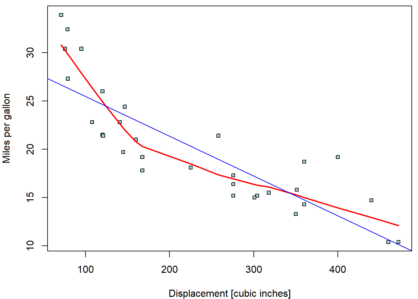
Apparently, linear trend describes the relationship poorly. The
lowess curve suggests more concave behaviour. Let us
consider other possible parametrizations (square root, quadratic
polynomial, cubic polynomial, piecewise-linear function with break in
170):
fit_disp <- list()
fit_disp[["line"]] <- lm(mpg ~ disp, data = mtcars)
fit_disp[["sqrt"]] <- lm(mpg ~ sqrt(disp), data = mtcars)
fit_disp[["log2"]] <- lm(mpg ~ log2(disp), data = mtcars)
fit_disp[["quad"]] <- lm(mpg ~ disp + disp^2, data = mtcars)                   # wrong!!!
fit_disp[["quad"]] <- lm(mpg ~ disp + I(disp^2), data = mtcars)                # this is correct!
fit_disp[["cube"]] <- lm(mpg ~ disp + I(disp^2) + I(disp^3), data = mtcars)
fit_disp[["hoc1"]] <- lm(mpg ~ pmin(disp-170, 0) + pmax(170, disp), data = mtcars)
fit_disp[["hoc2"]] <- lm(mpg ~ disp + pmax(170, disp), data = mtcars)
fit_disp[["flat"]] <- lm(mpg ~ pmin(170, disp), data = mtcars)

sum_disp <- lapply(fit_disp, summary) # summary for each model in the list
Notice that the additional power terms of disp have to
be wrapped by I(). The reason is that ^2 has
different meaning in formula notation (interactions).
Functions min and max return always only
one number - minimum or maximum from all given numbers. However, we wish
to compute minimum or maximum in vectorized form, always from two
numbers. This is done with pmin and pmax.
The models fit_disp_hoc1 and fit_disp_hoc2
are two equivalent parametrizations of the same piecewise-linear
function with break in 170. Both functions are forced to be continuous
in 170. We start with general description of two lines on two different
intervals, but then we need the same \(f(170)\) on both intervals.
In the first parametrization, beta coefficients (besides intercept) correspond to the slopes in different intervals. \[ f(x) = \left\{ \begin{aligned} a_1 + b_1 x, & \quad \text{for}\; x \in (-\infty, 170], \\ a_2 + b_2 x, & \quad \text{for}\; x \in [170, \infty), \end{aligned} \right. \quad \underset{\text{correction}}{\overset{\text{continuity}}{\Longrightarrow}} \quad f(x) = a_2 + b_1 \min (x-170, 0) + b_2 \max(170, x). \] In the second parametrization, the second coefficient is the slope in the first interval \((-\infty, 170]\) and the third coefficient describes the change from this slope to the slope in the other interval \([170, \infty)\). \[ f(x) = \left\{ \begin{aligned} a_1 + b x, & \quad \text{for}\; x \in (-\infty, 170], \\ a_2 + (b + \delta) x, & \quad \text{for}\; x \in [170, \infty), \end{aligned} \right. \quad \underset{\text{correction}}{\overset{\text{continuity}}{\Longrightarrow}} \quad f(x) = a_2 + b x + \delta \max(170, x). \] The intercept is the same in both cases as it corresponds to the intercept on the second interval. Compare:
sum_disp[["hoc1"]]##
## Call:
## lm(formula = mpg ~ pmin(disp - 170, 0) + pmax(170, disp), data = mtcars)
##
## Residuals:
## Min 1Q Median 3Q Max
## -3.5952 -1.6804 0.0674 1.1148 4.8660
##
## Coefficients:
## Estimate Std. Error t value Pr(>|t|)
## (Intercept) 22.176641 1.669701 13.282 7.41e-14 ***
## pmin(disp - 170, 0) -0.121801 0.015686 -7.765 1.46e-08 ***
## pmax(170, disp) -0.019607 0.005347 -3.667 0.00098 ***
## ---
## Signif. codes: 0 '***' 0.001 '**' 0.01 '*' 0.05 '.' 0.1 ' ' 1
##
## Residual standard error: 2.365 on 29 degrees of freedom
## Multiple R-squared: 0.856, Adjusted R-squared: 0.8461
## F-statistic: 86.19 on 2 and 29 DF, p-value: 6.263e-13sum_disp[["hoc2"]]##
## Call:
## lm(formula = mpg ~ disp + pmax(170, disp), data = mtcars)
##
## Residuals:
## Min 1Q Median 3Q Max
## -3.5952 -1.6804 0.0674 1.1148 4.8660
##
## Coefficients:
## Estimate Std. Error t value Pr(>|t|)
## (Intercept) 22.17664 1.66970 13.282 7.41e-14 ***
## disp -0.12180 0.01569 -7.765 1.46e-08 ***
## pmax(170, disp) 0.10219 0.01941 5.265 1.22e-05 ***
## ---
## Signif. codes: 0 '***' 0.001 '**' 0.01 '*' 0.05 '.' 0.1 ' ' 1
##
## Residual standard error: 2.365 on 29 degrees of freedom
## Multiple R-squared: 0.856, Adjusted R-squared: 0.8461
## F-statistic: 86.19 on 2 and 29 DF, p-value: 6.263e-13See? Intercept rows are both \(22.17664\). Next, \(-0.1218 + 0.10219 = -0.019607\)
The last model fit_disp_flat has some slope in the first
interval, but after 170 there is no trend only constant.
In order to plot the fitted curves we define the functions:
fun <- list()
fun[["line"]] <- function(beta, x){beta[1] + beta[2] * x}
fun[["sqrt"]] <- function(beta, x){beta[1] + beta[2] * sqrt(x)}
fun[["log2"]] <- function(beta, x){beta[1] + beta[2] * log2(x)}
fun[["quad"]] <- function(beta, x){beta[1] + beta[2] * x + beta[3] * x^2}
fun[["cube"]] <- function(beta, x){beta[1] + beta[2] * x + beta[3] * x^2 + beta[4] * x^3}
fun[["hoc1"]] <- function(beta, x){beta[1] + beta[2] * pmin(x-170, 0) + beta[3] * pmax(170, x)}
fun[["hoc2"]] <- function(beta, x){beta[1] + beta[2] * x + beta[3] * pmax(170, x)}
fun[["flat"]] <- function(beta, x){beta[1] + beta[2] * pmin(170, x)}
Now we plot all the fitted curves into one plot:
xgrid <- seq(min(mtcars$disp), max(mtcars$disp), length.out = 201)
COL <- c("blue", "purple", "orchid", "green", "darkgreen", "orange", "red", "peru")
names(COL) <- names(fit_disp)
nice_labels <- c("line", "square root", expression(log[2]),
                 "quadratic", "cubic",
                 "hockey 1", "hockey 2", "flat hockey")

par(mfrow = c(1,1), mar = c(4,4,0.5,0.5))
plot(mpg ~ disp, data = mtcars,
     xlab = "Displacement [cubic inches]", ylab = "Miles per gallon",
     pch = 22, cex = 0.8, bg = "lightblue")
abline(v = 170, col = "grey", lty = 3)
# now add the estimated curves
for(curve in names(fit_disp)){
  lines(xgrid, fun[[curve]](coef(fit_disp[[curve]]), xgrid),
        col = COL[curve], lwd = 2, lty = ifelse(curve == "hoc2", 2, 1))
}
legend("topright", legend = nice_labels, bty = "n",
       col = COL, lty = c(1,1,1,1,1,2,1), lwd = 2)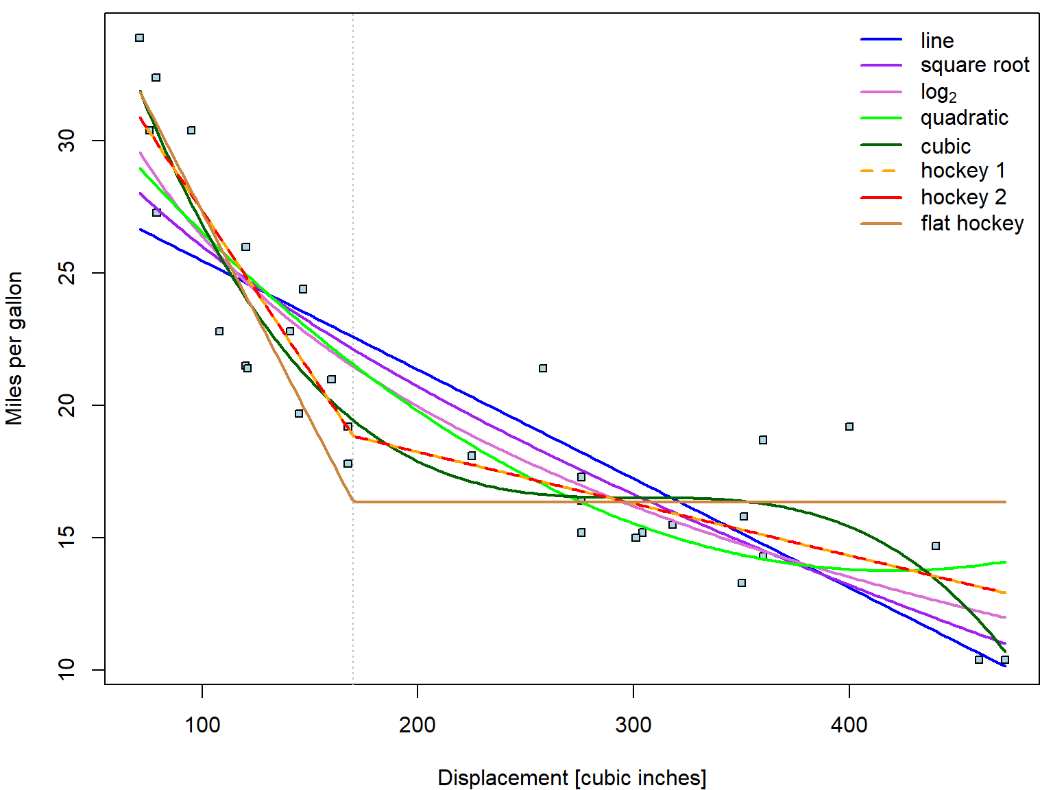
You actually do not have to define the functions on your own. There
is always an option to use predict function to estimate the
fitted value fit given grid of newdata
covariates.
pred_disp <- lapply(fit_disp, predict, newdata = data.frame(disp = xgrid))The predict function will work this way as long as disp
is transformed directly within the model formula. If you would define
disp2 = disp^2, then your newdata need to
contain disp2 as well. See? The results are the same:
par(mfrow = c(1,1), mar = c(4,4,0.5,0.5))
plot(mpg ~ disp, data = mtcars,
     xlab = "Displacement [cubic inches]", ylab = "Miles per gallon",
     pch = 22, cex = 0.8, bg = "lightblue")
abline(v = 170, col = "grey", lty = 3)
# now add the estimated curves
for(curve in names(fit_disp)){
  lines(xgrid, pred_disp[[curve]],
        col = COL[curve], lwd = 2, lty = ifelse(curve == "hoc2", 2, 1))
}
legend("topright", legend = nice_labels, bty = "n",
       col = COL, lty = c(1,1,1,1,1,2,1), lwd = 2)
How do we choose suitable transformation?
- Visual appeal (above),
- Satisfactory visual diagnostic tools (will be covered in more details later in Exercise 8)
- Proportion of explained variability - by \(R^2\) (always higher for model compared to its submodel),
- Overall F-test p-value (takes number of coefficients required into account),
- Model selection criteria (AIC, BIC) - to avoid over-fitting,
- Submodel tests (if valid)
table <- data.frame(R2 = unlist(lapply(sum_disp, function(s){s$r.squared})),
                    adjR2 = unlist(lapply(sum_disp, function(s){s$adj.r.squared})),
                    Fpval = unlist(lapply(sum_disp, function(s){
                      pf(s$fstatistic["value"], df1 = s$fstatistic["numdf"],
                         df2 = s$fstatistic["dendf"], lower.tail = FALSE
                         )})),
                    AIC = unlist(lapply(fit_disp, AIC)))

library(knitr)
kable(table, digits = 15)| R2 | adjR2 | Fpval | AIC | |
|---|---|---|---|---|
| line | 0.7183433 | 0.7089548 | 9.38033e-10 | 170.2094 |
| sqrt | 0.7756108 | 0.7681311 | 2.99310e-11 | 162.9356 |
| log2 | 0.8228521 | 0.8169471 | 8.40000e-13 | 155.3709 |
| quad | 0.7927323 | 0.7784380 | 1.22944e-10 | 162.3957 |
| cube | 0.8770603 | 0.8638881 | 7.35000e-13 | 147.6816 |
| hoc1 | 0.8559880 | 0.8460561 | 6.26000e-13 | 150.7440 |
| hoc2 | 0.8559880 | 0.8460561 | 6.26000e-13 | 150.7440 |
| flat | 0.7892135 | 0.7821872 | 1.16210e-11 | 160.9344 |
par(mfrow = c(2,4), mar = c(4,4,2,0.5))
for(curve in names(fit_disp)){
  plot(fit_disp[[curve]], which = 1)
  legend("topright", legend = curve)
}
Individual work
- Choose the best fitting trend.
- Repeat for other numeric covariates -
hpanddrat. - Fit a model with the chosen parametrizations of all three covariates.