Non-parametric estimation of cumulative hazard and survival function

Lecture revision: blackboard notes.

Theory

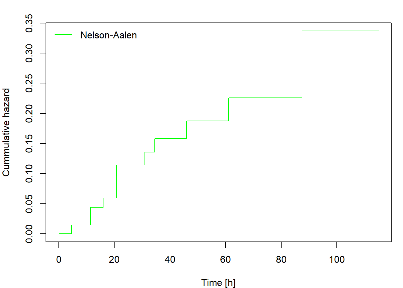
The cumulative hazard can be estimated non-parametrically by the Nelson-Aalen estimator defined as

\[ \widehat{\Lambda}(t)=\int_0^t\frac{\,\mathrm{d} \overline{N}(u)}{\overline{Y}(u)}= \sum_{\{i: t_i\leq t\}} \frac{\Delta\overline{N}(t_i)}{\overline{Y}(t_i)}, \] where \(0<t_1<t_2<\cdots<t_d\) are ordered distinct failure times.

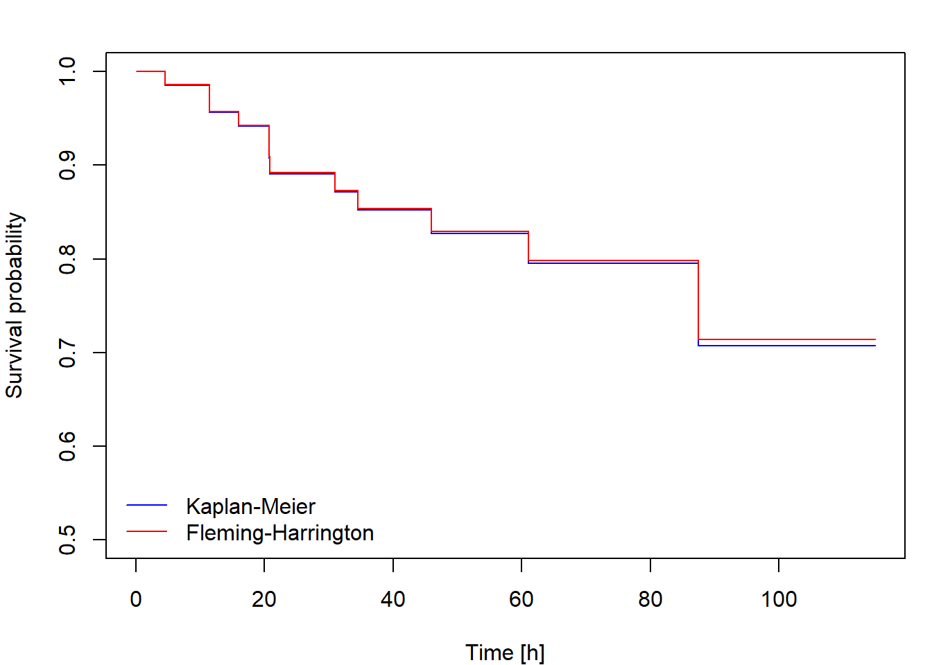
The Kaplan-Meier [KM] estimator of the survival function is \[ \widehat{S}(t)=\prod_{\{i: t_i\leq t\}}\biggl[1-\frac{\Delta\overline{N}(t_i)}{\overline{Y}(t_i)}\biggr]. \] If the distribution of \(T_i\) is continuous, one could define an alternative survival function estimator using the relationship \(S(t)=\exp\{-\Lambda(t)\}\) applied to the Nelson-Aalen estimator, that is \[ \widehat{S}_*(t)=\exp\{-\widehat{\Lambda}(t)\}=\prod_{\{i: t_i\leq t\}}\exp\biggl\{-\frac{\Delta\overline{N}(t_i)}{\overline{Y}(t_i)}\biggr\}. \] This is called the Fleming-Harrington [FH] estimator (sometimes also the Breslow estimator). Because \(\exp\{-h\}\approx 1-h\) for small \(h\), the difference between the KM and FH estimators is small unless the risk set size \(\overline{Y}(u)\) is not large enough, which happens at the largest failure times. The FH estimator is not suitable for discrete data, while the KM estimator works well for both discrete and continuous cases.

Understanding the formulae

The dataset fans [Nelson, Journal of Quality Technology, 1:27-52, 1969] comes from an engineering study of the time to failure of diesel generator fans. Seventy generators were studied. For each one, the number of hours of running time from its first being put into service until fan failure or until the end of the study (whichever came first) was recorded.

The data is available in the RData format from this link. The dataframe is called fans, the variable fans$time includes the censored failure time \(X_i\) (in hours), the variable fans$fail is the failure indicator \(\delta_i\).

We will use this dataset to demonstrate the calculation of cumulative hazard and survival function estimates.

Task 1

Using ordinary R functions (table, cumsum, cumprod, rev, …, but not functions from the survival package), calculate and print the following table:

\(i\)	\(t_i\)	\(d_i\)	\(y_i\)	\(d_i/y_i\)	\(L_i\)	\(S_i\)	\(S^*_i\)
1	…	…	…	…	…	…	…
…	…	…	…	…	…	…	…
d	…	…	…	…	…	…	…

where \(i\) is the order of the failures, \(t_i\) is the ordered failure time, \(d_i=\Delta\overline{N}(t_i)\), \(y_i=\overline{Y}(t_i)\), \(L_i=\widehat{\Lambda}(t_i)\), \(S_i=\widehat{S}(t_i)\), and \(S^*_i=\widehat{S}_*(t_i)\).

Then plot the cumulative hazard estimator and both survival function estimators.

Show final table

Show NA plot

Show KM and FH plot

Show nicer and separated KM and FH plots

##       t d  y        d_y          L         S     Sstar
## 1   0.0 0 70 0.00000000 0.00000000 1.0000000 1.0000000
## 2   4.5 1 70 0.01428571 0.01428571 0.9857143 0.9858158
## 3  11.5 2 68 0.02941176 0.04369748 0.9567227 0.9572435
## 4  16.0 1 65 0.01538462 0.05908209 0.9420039 0.9426294
## 5  20.7 2 55 0.03636364 0.09544573 0.9077492 0.9089677
## 6  20.8 1 53 0.01886792 0.11431366 0.8906218 0.8919781
## 7  31.0 1 47 0.02127660 0.13559025 0.8716724 0.8732004
## 8  34.5 1 45 0.02222222 0.15781247 0.8523019 0.8540099
## 9  46.0 1 34 0.02941176 0.18722424 0.8272342 0.8292578
## 10 61.0 1 26 0.03846154 0.22568578 0.7954175 0.7979688
## 11 87.5 1  9 0.11111111 0.33679689 0.7070378 0.7140539

Calculating the estimators using library(survival)

The basic functions for censored data analysis are available in R package survival. Censored data are entered as special survival objects created in this way:

library("survival")
Surv(time, del)
## see help("Surv")
# used as a response variable in a model formula
# right censoring is set as default

where time is a numeric vector containing the censored failure times and del is a numeric vector containing failure indicators (1 = failure, 0 = censored). Survival objects are used as input to functions providing analysis of censored data.

Survival function estimates are calculated by the function survfit. The most rudimentary use of this function is

fit <- survfit(Surv(time, del) ~ 1, data = data)

This calculates the KM estimator. The FH estimator is obtained by adding an option type

fit <- survfit(Surv(time, del) ~ 1, type = "fleming", data = data)

The results can be plotted easily by calling

plot(fit)

For demonstration, we will use the dataset aml included in library("survival"). Survival in patients with Acute Myelogenous Leukemia. The question at the time was whether the standard course of chemotherapy should be extended (‘maintenance’) for additional cycles.

print(aml)

##    time status             x
## 1     9      1    Maintained
## 2    13      1    Maintained
## 3    13      0    Maintained
## 4    18      1    Maintained
## 5    23      1    Maintained
## 6    28      0    Maintained
## 7    31      1    Maintained
## 8    34      1    Maintained
## 9    45      0    Maintained
## 10   48      1    Maintained
## 11  161      0    Maintained
## 12    5      1 Nonmaintained
## 13    5      1 Nonmaintained
## 14    8      1 Nonmaintained
## 15    8      1 Nonmaintained
## 16   12      1 Nonmaintained
## 17   16      0 Nonmaintained
## 18   23      1 Nonmaintained
## 19   27      1 Nonmaintained
## 20   30      1 Nonmaintained
## 21   33      1 Nonmaintained
## 22   43      1 Nonmaintained
## 23   45      1 Nonmaintained

We get a full description of our estimates of survival function by summary applied to survfit object:

fit_KM <- survfit(Surv(time, status) ~ 1, data = aml)
summary(fit_KM)

## Call: survfit(formula = Surv(time, status) ~ 1, data = aml)
## 
##  time n.risk n.event survival std.err lower 95% CI upper 95% CI
##     5     23       2   0.9130  0.0588       0.8049        1.000
##     8     21       2   0.8261  0.0790       0.6848        0.996
##     9     19       1   0.7826  0.0860       0.6310        0.971
##    12     18       1   0.7391  0.0916       0.5798        0.942
##    13     17       1   0.6957  0.0959       0.5309        0.912
##    18     14       1   0.6460  0.1011       0.4753        0.878
##    23     13       2   0.5466  0.1073       0.3721        0.803
##    27     11       1   0.4969  0.1084       0.3240        0.762
##    30      9       1   0.4417  0.1095       0.2717        0.718
##    31      8       1   0.3865  0.1089       0.2225        0.671
##    33      7       1   0.3313  0.1064       0.1765        0.622
##    34      6       1   0.2761  0.1020       0.1338        0.569
##    43      5       1   0.2208  0.0954       0.0947        0.515
##    45      4       1   0.1656  0.0860       0.0598        0.458
##    48      2       1   0.0828  0.0727       0.0148        0.462

We calculate and plot KM and FH estimates like this

fit_FH <- survfit(Surv(time, status) ~ 1, type = "fleming", data = aml)

par(mar=c(4, 4, 1, 1))
plot(fit_KM, conf.int = FALSE, col = "blue",
     xlab = "Time", ylab = "Survival probability")
lines(fit_FH, conf.int = FALSE, col = "red")
legend("topright", c("Kaplan-Meier", "Fleming-Harrington"), 
       col = c("blue", "red"), lty = 1, bty = "n")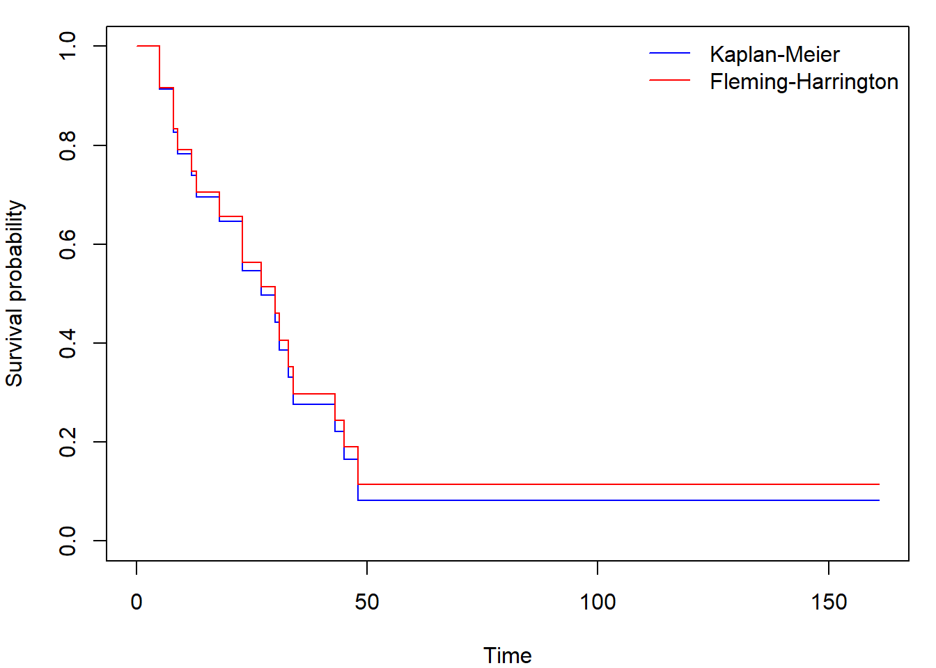

We suppressed the plotting of the confidence intervals.

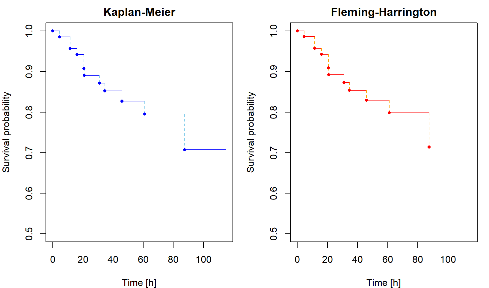
Sometimes you can come across figures with crosses at times where an observation was censored (set mark.time = TRUE, default mark is +):

par(mar = c(4, 4, 1, 1))
plot(fit_KM, conf.int = FALSE, col = "blue", mark.time = TRUE,
     xlab = "Time", ylab = "Survival probability")
legend("topright","Kaplan-Meier", 
       col = "blue", lty = 1, bty = "n")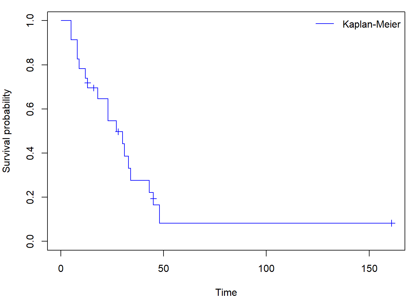

Using the formula notation, we can easily create and plot separate curves for two distinct subgroups of observations (declared by the factor variable x within model formula instead of 1):

fit_gr <- survfit(Surv(time, status) ~ x, data = aml)
par(mar = c(4, 4, 1, 1))
plot(fit_gr, col = c("green", "magenta"), xlab = "Time", ylab = "Survival probability")
legend("topright", levels(aml$x), col = c("green","magenta"), lty = 1, bty = "n")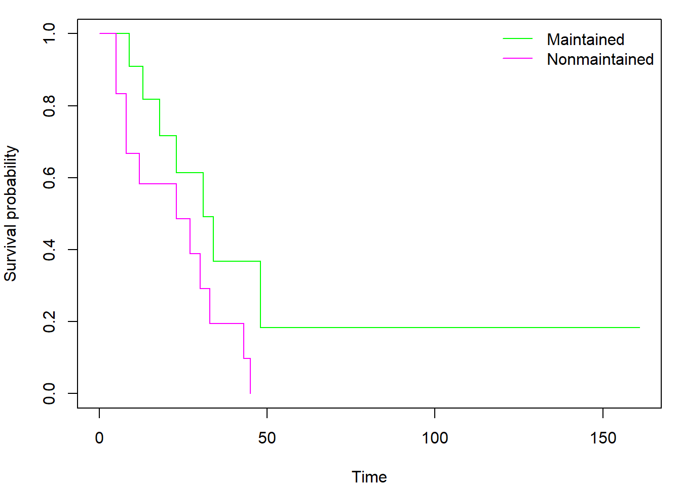

It is interesting to investigate the contents of the survfit object by calling str(fit_KM). By doing so, you may discover also the Nelson-Aalen estimator of cumulative hazard function hidden in $cumhaz. Regardless of selected type (kaplan or fleming) $cumhaz always contains the Nelson-Aalen estimator. If you need cumulative hazard estimator derived from Kaplan-Meier estimator of survival function you have to use the transformation \(\Lambda(t) = - \log \left( S(t) \right)\). You can also easily plot the cumulative hazard function(s) by adding fun = "cumhaz" into the plot command (see help(plot.survfit) for other uses of fun parameter):

par(mar = c(4, 4, 1, 1))
plot(fit_gr, col = c("green", "magenta"), xlab = "Time", ylab = "Cumulative hazard function",
     fun = "cumhaz")
legend("topright", levels(aml$x), col = c("green","magenta"), lty = 1, bty = "n")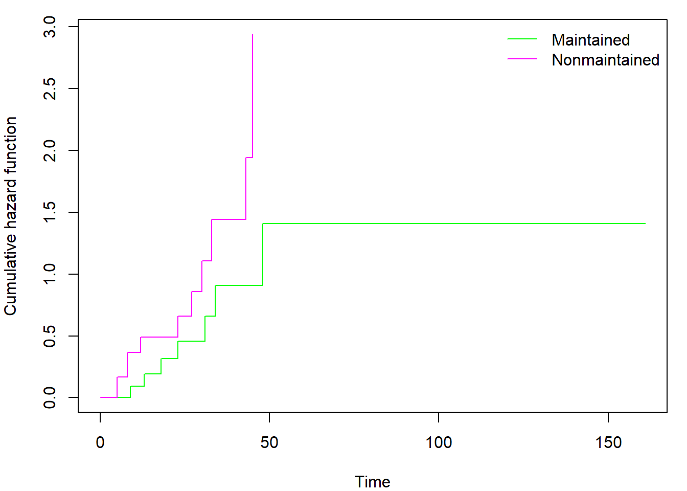

You can also use library("ggplot2") in cooperation with library("survminer") to obtain nicer plots:

library("survminer")
library("ggplot2")
ggsurvplot(fit_gr, conf.int = FALSE, censor= TRUE,
           ggtheme = theme_minimal())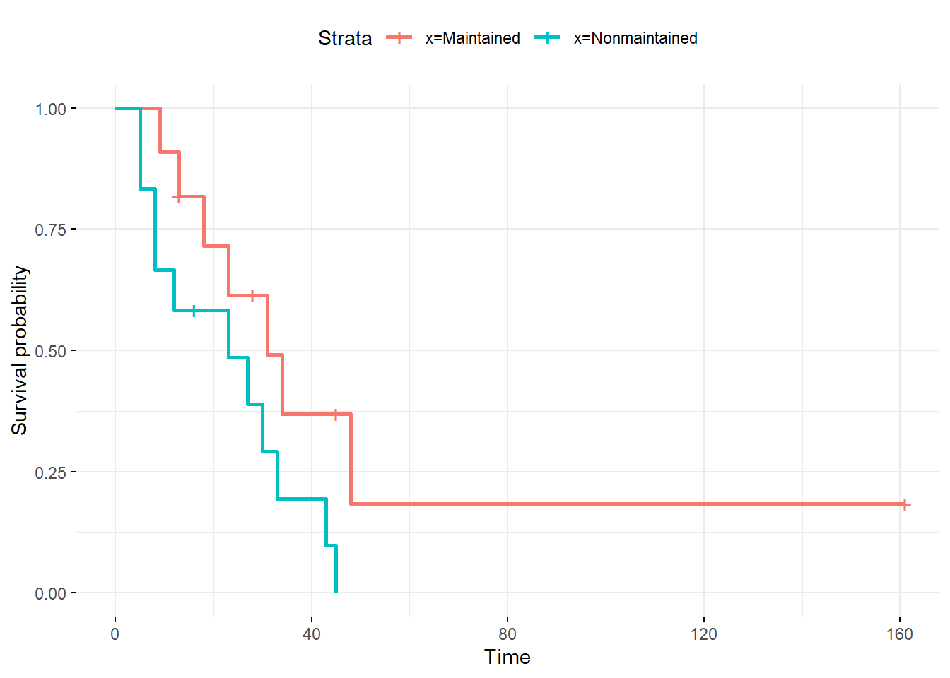

Homework assignment

Calculate and plot the cumulative hazard estimator and both survival function estimators for fans data using the function survfit. Compare the results to those you obtained in Task 1. Include the code, output and comments in your report.

Advice: Implement your own function for creating nicely looking step-functions. You will surely use it in a near future.

• Deadline for report: 25th November 2024, 05:55 CET.

Theoretical Task 1 (voluntary)

Show that the Nelson-Aalen estimator satisfies the equation \[ \sum_{i=1}^n \widehat{\Lambda}(X_i)=\sum_{i=1}^n \delta_i. \]

Theoretical Task 2 (voluntary)

Show that under absence of censored data the Kaplan-Meier estimator becomes classical empirical estimator: \[ \widehat{S}(t) = \prod\limits_{\{j: t_j \leq t\}} \left[1 - \dfrac{\Delta\overline{N}(t_j)}{\overline{Y}(t_j)}\right] = \frac{1}{n}\sum \limits_{i=1}^n \mathbb{I}(X_i > t), \quad \forall t >0. \]