Parametric regression models for censored data

Lecture revision: blackboard notes.

PBC (Primary Biliary Cirrhosis) dataset

This data is from the Mayo Clinic trial in primary biliary cirrhosis (PBC) of the liver conducted between 1974 and 1984. A total of 424 PBC patients, referred to Mayo Clinic during that ten-year interval, met eligibility criteria for the randomized placebo controlled trial of the drug D-penicillamine. The first 312 cases in the data set participated in the randomized trial and contain largely complete data. The additional 112 cases did not participate in the clinical trial, but consented to have basic measurements recorded and to be followed for survival. Six of those cases were lost to follow-up shortly after diagnosis, so the data here are on an additional 106 cases as well as the 312 randomized participants.

library(survival)
dim(pbc)

## [1] 418  25

pbc <- pbc[, c("id", "time", "status", "trt", "sex", "edema", "bili", "albumin", "platelet")]
# id = case number
# time = number of days between registration and the earlier of death, transplantion, or study analysis in July, 1986
# status = status at endpoint, 0/1/2 for censored, transplant, dead
# trt = 1/2/NA for D-penicillamin, placebo, not randomised
# sex =  m/f
# edema = 0 no edema, 0.5 untreated or successfully treated, 1 edema despite diuretic therapy
# bili = serum bilirunbin (mg/dl)
# albumin = serum albumin (g/dl)
# platelet = platelet count
head(pbc)

##   id time status trt sex edema bili albumin platelet
## 1  1  400      2   1   f   1.0 14.5    2.60      190
## 2  2 4500      0   1   f   0.0  1.1    4.14      221
## 3  3 1012      2   1   m   0.5  1.4    3.48      151
## 4  4 1925      2   1   f   0.5  1.8    2.54      183
## 5  5 1504      1   2   f   0.0  3.4    3.53      136
## 6  6 2503      2   2   f   0.0  0.8    3.98       NA

summary(pbc)

##        id             time          status            trt        sex         edema             bili       
##  Min.   :  1.0   Min.   :  41   Min.   :0.0000   Min.   :1.000   m: 44   Min.   :0.0000   Min.   : 0.300  
##  1st Qu.:105.2   1st Qu.:1093   1st Qu.:0.0000   1st Qu.:1.000   f:374   1st Qu.:0.0000   1st Qu.: 0.800  
##  Median :209.5   Median :1730   Median :0.0000   Median :1.000           Median :0.0000   Median : 1.400  
##  Mean   :209.5   Mean   :1918   Mean   :0.8301   Mean   :1.494           Mean   :0.1005   Mean   : 3.221  
##  3rd Qu.:313.8   3rd Qu.:2614   3rd Qu.:2.0000   3rd Qu.:2.000           3rd Qu.:0.0000   3rd Qu.: 3.400  
##  Max.   :418.0   Max.   :4795   Max.   :2.0000   Max.   :2.000           Max.   :1.0000   Max.   :28.000  
##                                                  NA's   :106                                              
##     albumin         platelet    
##  Min.   :1.960   Min.   : 62.0  
##  1st Qu.:3.243   1st Qu.:188.5  
##  Median :3.530   Median :251.0  
##  Mean   :3.497   Mean   :257.0  
##  3rd Qu.:3.770   3rd Qu.:318.0  
##  Max.   :4.640   Max.   :721.0  
##                  NA's   :11

Exponential regression with arbitrary random censoring

Let us suppose the following model. We are interested in the distribution of survival time of a patient denoted by \(T\). \(C\) will denote the (censoring) time when the patient had (or would have had) transplantation or the time for which he/she has been observed. What we actually measure is the time of the event, which comes first, i.e. \(X = \min \{T, C \}\) (variable time). We also know \(\delta\) - the indicator of what event actually happened (variable status). Our data consist of \(n\) = 418 triplets \(\left(X_i, \delta_i, \mathbf{Z}_i\right)\), where \(\mathbf{Z}_i\) are other measured covariates.

We suppose that these triplets are stochastically independent of each other, censoring times \(C_i\) are arbitrary and independent of survival times \(T_i\), however, we suppose that \[T_i | \mathbf{Z}_i \sim \mathsf{Exp} \left(\lambda(\mathbf{Z}_i, \boldsymbol\beta) \right), \qquad \text{where} \; \lambda(\mathbf{Z}, \boldsymbol \beta) = \lambda_0 \exp \left\{ \boldsymbol\beta^{\mathsf{T}} \mathbf{Z} \right\} \] are individual hazards arising from linear combination of given covariates. \(\lambda_0\) is called the baseline hazard (\(\lambda = \lambda_0 \Leftrightarrow \mathbf{Z}_i = \mathbf{0}\)). For identifiability purposes we do not allow intercept among covariates \(\mathbf{Z}_i\) (in this notation). The goal is to estimate unknown coefficients \(\boldsymbol \beta\) in order to describe the influence of covariates on the hazard.

We can fit this model in R using glm function with appropriate setting (see lecture notes).

Usage of glm function

The following must be done:

• Response variable must be set to \(\delta\) indicator.
• Choose appropriate set of covariates (intercept is automatically included).
  • Intercept term corresponds to \(\log \lambda_0\).
• Add + offset(log(time)) into the model formula.
• Set family = poisson (with canonical \(\log\) link).

However, even if we proceed according to these rules, the following model is still invalid:

fit_cens_WRONG <- glm(status ~ trt + sex + edema + bili + albumin + platelet + offset(log(time)), family=poisson, data = pbc)
summary(fit_cens_WRONG)

## 
## Call:
## glm(formula = status ~ trt + sex + edema + bili + albumin + platelet + 
##     offset(log(time)), family = poisson, data = pbc)
## 
## Deviance Residuals: 
##     Min       1Q   Median       3Q      Max  
## -2.7052  -1.1500  -0.8297   1.0742   3.7721  
## 
## Coefficients:
##               Estimate Std. Error z value Pr(>|z|)    
## (Intercept) -3.7767641  0.5943777  -6.354 2.10e-10 ***
## trt         -0.1222921  0.1241319  -0.985 0.324536    
## sexf        -0.7083493  0.1657342  -4.274 1.92e-05 ***
## edema        0.8306849  0.2182798   3.806 0.000141 ***
## bili         0.0982134  0.0098939   9.927  < 2e-16 ***
## albumin     -0.9490988  0.1564953  -6.065 1.32e-09 ***
## platelet    -0.0010431  0.0006906  -1.511 0.130910    
## ---
## Signif. codes:  0 '***' 0.001 '**' 0.01 '*' 0.05 '.' 0.1 ' ' 1
## 
## (Dispersion parameter for poisson family taken to be 1)
## 
##     Null deviance: 776.37  on 307  degrees of freedom
## Residual deviance: 533.22  on 301  degrees of freedom
##   (110 observations deleted due to missingness)
## AIC: 909.32
## 
## Number of Fisher Scoring iterations: 6

Task

Find out what is wrong with this model and make necessary changes.

You should correct the following: Show hint

• Define delta <- (status == 2) and use it instead of status.
• Factorize seemingly categorical variables.
• Deal with presence of NA values (trt and platelet).
• \(\pm\) Transform continuous variables.

After needed changes we get the following results:

fit_cens <- glm(delta ~ ftrt + fsex + fedema + bili + albumin + platelet + offset(log(time)), family=poisson, data = subdata)
summary(fit_cens)

## 
## Call:
## glm(formula = delta ~ ftrt + fsex + fedema + bili + albumin + 
##     platelet + offset(log(time)), family = poisson, data = subdata)
## 
## Deviance Residuals: 
##     Min       1Q   Median       3Q      Max  
## -1.9482  -0.7927  -0.5976   0.7868   2.6869  
## 
## Coefficients:
##                      Estimate Std. Error z value Pr(>|z|)    
## (Intercept)        -5.1171852  0.7756655  -6.597 4.19e-11 ***
## ftrtD-penicillamin  0.1533012  0.1860559   0.824  0.40997    
## ftrtnot_rand       -0.0067883  0.2341321  -0.029  0.97687    
## fsexfemale         -0.5580839  0.2285004  -2.442  0.01459 *  
## fedemaappeared      0.3791800  0.2399243   1.580  0.11401    
## fedemaserious       1.0097446  0.3074263   3.285  0.00102 ** 
## bili                0.1024013  0.0131163   7.807 5.85e-15 ***
## albumin            -0.8922870  0.2027481  -4.401 1.08e-05 ***
## platelet           -0.0012364  0.0008936  -1.384  0.16649    
## ---
## Signif. codes:  0 '***' 0.001 '**' 0.01 '*' 0.05 '.' 0.1 ' ' 1
## 
## (Dispersion parameter for poisson family taken to be 1)
## 
##     Null deviance: 529.71  on 406  degrees of freedom
## Residual deviance: 387.11  on 398  degrees of freedom
## AIC: 715.11
## 
## Number of Fisher Scoring iterations: 6

Classical functions as anova, drop1, add1 can be used for finding a suitable model:

anova(fit_cens, test = "Chisq")
drop1(fit_cens, test = "Chisq")
add1(fit_cens, scope = c("ftrt:albumin", "fedema:bili"), test = "Chisq")

Homework assignment

Find a suitable model for \(\lambda(\mathbf{Z}, \boldsymbol\beta)\) based on pbc data and interpret it. Write also down all the assumptions of the used probabilistic model including the formula for \(\lambda(\mathbf{Z}, \boldsymbol\beta)\).

• Deadline for report: Monday 14th November 9:00

Maybe useful function for determining useful parametrization of continuous variables:

variables <- c("bili", "albumin", "platelet")
PlotCoefFactor <- function(variable, ngroups = 10){
  # variable must be in the data
  if(!is.element(variable, colnames(subdata))){stop(paste("variable", variable, "is not included in subdata!"))}
  # ngroups >= 2 !!!!
  if(ngroups < 2){stop("ngroups has to be at least 2!")}
  othervar <- setdiff(variables, variable)
  qq <- quantile(subdata[,variable], probs = seq(0,1,length.out = ngroups+1))
  ff <- cut(subdata[,variable], breaks = c(-Inf, qq[2:ngroups], Inf))
  model <- glm(as.formula(paste("delta ~ ftrt + fsex + fedema + ff +",
                                paste(setdiff(variables, variable), collapse = " + "), 
                                " + offset(log(time))", sep = "")), 
               family = poisson, data = subdata)
  yy <- c(0, # coefficient for the first (reference) group
          model$coefficients[grep("ff", names(model$coefficients))]) 
  xx <- (qq[1:ngroups]+qq[2:(ngroups+1)])/2
  plot(yy ~ xx, 
       type = "b", 
       xlab = variable, 
       ylab = "Coefficient",
       cex = summary(ff)/max(summary(ff))*2+0.5)
  }

# For example bili
par(mar = c(4,4,1,1))
PlotCoefFactor("bili")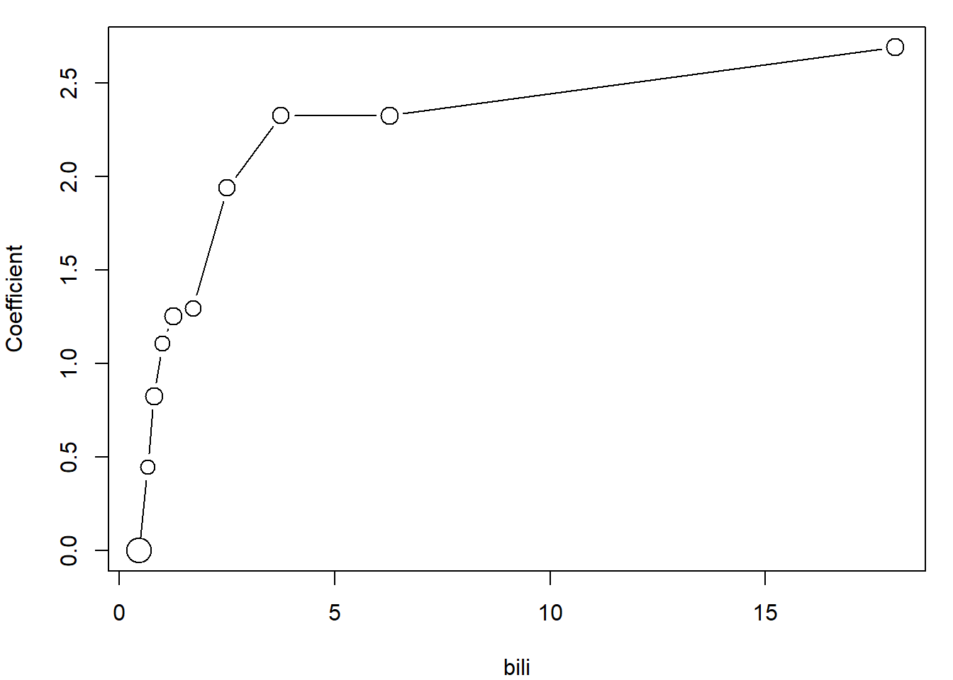

Ignoring censoring

Suppose we were not given the \(\delta\)-indicator and believe that variable time always represents the time of death of patient. We would still suppose the same model \[X_i = T_i | \mathbf{Z}_i \sim \mathsf{Exp} \left(\lambda(\mathbf{Z}_i, \boldsymbol\beta) \right), \qquad \text{where} \; \lambda(\mathbf{Z}, \boldsymbol \beta) = \lambda_0 \exp \left\{ \boldsymbol\beta^{\mathsf{T}} \mathbf{Z} \right\}. \] This model is exponential regression that belongs to Gamma family of GLM and can be fitted directly using glm function in two ways.

family = Gamma, link = "log" and dispersion = 1

fit_exp_regr1 <- glm(time ~ ftrt + fsex + fedema + bili + albumin + platelet, family = Gamma(link = "log"), data = subdata)
summary(fit_exp_regr1, dispersion = 1)

## 
## Call:
## glm(formula = time ~ ftrt + fsex + fedema + bili + albumin + 
##     platelet, family = Gamma(link = "log"), data = subdata)
## 
## Deviance Residuals: 
##      Min        1Q    Median        3Q       Max  
## -2.18365  -0.42103  -0.05654   0.26064   1.58953  
## 
## Coefficients:
##                      Estimate Std. Error z value Pr(>|z|)    
## (Intercept)         6.0701346  0.5103532  11.894  < 2e-16 ***
## ftrtD-penicillamin -0.0225165  0.1145596  -0.197 0.844181    
## ftrtnot_rand       -0.1896422  0.1322375  -1.434 0.151543    
## fsexfemale          0.0373071  0.1624863   0.230 0.818401    
## fedemaappeared     -0.1099104  0.1658821  -0.663 0.507599    
## fedemaserious      -0.6979133  0.2587123  -2.698 0.006983 ** 
## bili               -0.0474816  0.0122692  -3.870 0.000109 ***
## albumin             0.4358234  0.1296959   3.360 0.000778 ***
## platelet            0.0004048  0.0005244   0.772 0.440126    
## ---
## Signif. codes:  0 '***' 0.001 '**' 0.01 '*' 0.05 '.' 0.1 ' ' 1
## 
## (Dispersion parameter for Gamma family taken to be 1)
## 
##     Null deviance: 199.30  on 406  degrees of freedom
## Residual deviance: 140.67  on 398  degrees of freedom
## AIC: 6709.2
## 
## Number of Fisher Scoring iterations: 7

Replace delta by vector of ones

fit_exp_regr2 <- glm(rep(1,dim(subdata)[1]) ~ ftrt + fsex + fedema + bili + albumin + platelet + offset(log(time)), family=poisson, data = subdata)
summary(fit_exp_regr2)

## 
## Call:
## glm(formula = rep(1, dim(subdata)[1]) ~ ftrt + fsex + fedema + 
##     bili + albumin + platelet + offset(log(time)), family = poisson, 
##     data = subdata)
## 
## Deviance Residuals: 
##      Min        1Q    Median        3Q       Max  
## -1.58954  -0.26064   0.05654   0.42103   2.18365  
## 
## Coefficients:
##                      Estimate Std. Error z value Pr(>|z|)    
## (Intercept)        -6.0701177  0.5067504 -11.979  < 2e-16 ***
## ftrtD-penicillamin  0.0225142  0.1151535   0.196 0.844990    
## ftrtnot_rand        0.1896398  0.1334791   1.421 0.155391    
## fsexfemale         -0.0373090  0.1632920  -0.228 0.819273    
## fedemaappeared      0.1099083  0.1676906   0.655 0.512195    
## fedemaserious       0.6979189  0.2570672   2.715 0.006629 ** 
## bili                0.0474806  0.0113436   4.186 2.84e-05 ***
## albumin            -0.4358263  0.1292282  -3.373 0.000745 ***
## platelet           -0.0004048  0.0005343  -0.758 0.448616    
## ---
## Signif. codes:  0 '***' 0.001 '**' 0.01 '*' 0.05 '.' 0.1 ' ' 1
## 
## (Dispersion parameter for poisson family taken to be 1)
## 
##     Null deviance: 199.30  on 406  degrees of freedom
## Residual deviance: 140.67  on 398  degrees of freedom
## AIC: 972.67
## 
## Number of Fisher Scoring iterations: 5

These approaches yield (almost) the same estimates except for change of sign. However, what is the comparison of these results to the model with censoring times?

Small simulation study

What would happen if the censoring was ignored and the parameters would be estimated based on the model \[X_i = T_i \sim \mathsf{Exp}\left(\lambda_i\right), \qquad \lambda_i = \lambda_0 \exp \left\{\beta Z_i\right\},\] however, the true model would be the one with censoring? See the script ignoring_censoring.R.