Actuarial (lifetable) estimator of the survival
Jan Vávra
Exercise 3 (21st November 2022)
Revision: Kaplan-Meier estimator
The Kaplan-Meier [KM] estimator of the survival function \[ \widehat{S}(t) = \prod_{\{i: t_i\leq t\}}\biggl[1-\frac{\Delta\overline{N}(t_i)}{\overline{Y}(t_i)}\biggr] = \widehat{S}(t-) \cdot \biggl[1-\frac{\Delta\overline{N}(t)}{\overline{Y}(t)}\biggr] \] is motivated by decomposition of the survival probability by chain rule. If the survival distribution is continuous the increment process \(\Delta \overline{N}\) attains only values 0 (no death at time \(t\)) or 1 (exactly one death at time \(t\)). In practice, however, time is not measured continuously or with necessary precision. Then ties begin to occur in the data and more death at the same time can be observed. If the ties come “accidentally”, for example, by rounding the true value, and its presence is rare, then [KM] works still fine. However, when the grouping of time (now rather categorical than continuous) comes from the design of the study itself, the resulting estimate could possibly result in unsatisfactory outputs.
Several methods for adjusting this fact have been proposed, we will introduce the Lifetable or Actuarial estimator.
Lifetable or actuarial estimator
Applies when the event times are grouped
Our goal is still to estimate the survival function, hazard, and density function, but this is complicated by the fact that we don’t know exactly when during each time interval an event occurs.
Notation:
- the \(j\)-th time interval is \([t_{j-1},t_j)\),
- \(c_j\) - the number of censorings in the \(j\)-th interval,
- \(d_j\) - the number of failures (deaths) in the \(j\)-th interval,
- \(r_j\) - the number of units entering the interval.
We could apply the K-M formula directly. However, it treats the problem as though it were in discrete time, with events happening only at endpoints of intervals. But the true events event times lie somewhere within the preceding interval. In fact, what we are trying to calculate here is the conditional probability of dying within the interval, given survival to the beginning of it.
We now make the assumption that the censoring process is such that the censored survival times occur uniformly throughout the \(j\)-th interval. So, we can assume that censorings occur on average halfway through the interval: \[ r_j'=r_j-c_j/2. \] I.e., average number of individuals who are at risk during this interval. The assumption yields the Actuarial Estimator. It is appropriate if censorings occur uniformly throughout the interval. This assumption is sometimes known as the actuarial assumption.
The event that an individual survives beyond \([t_{j-1},t_j)\) is equivalent to the event that an individual survives beyond \([t_{0},t_1)\) and … and that an individual survives beyond \([t_{j-2},t_{j-1})\) and that an individual survives beyond \([t_{j-1},t_j)\). Let us define the following quantities:
- \(P_j=P\{\mbox{an individual survives beyond }[t_{j-1},t_j)\}\),
- \(p_j=P\{\mbox{an individual survives beyond }[t_{j-1},t_j) |\mbox{ he survives beyond }[t_{j-2},t_{j-1})\}, \quad j>1\),
- \(p_1=P_1.\)
Then by chain rule, \[ P_j=p_1 \cdot \; \cdots \; \cdot p_j. \] The conditional probability of an death in \([t_{j-1},t_j)\) given that the individual survives beyond \([t_{j-2},t_{j-1})\) is estimated by \[ d_j/r_j'. \] Thus, \(p_j\) is estimated by \[ \frac{r_j'-d_j}{r_j'}. \] So, the actuarial (lifetime) estimate of the survival function is \[ \widehat{S}(t)=\prod_{j=1}^{k-1}\frac{r_j'-d_j}{r_j'} \qquad \text{for } t_{k-1} \leq t < t_{k}. \]
Remarks:
- Because the intervals are defined as \([t_{j-1}, t_j)\), the first interval typically starts with \(t_0 = 0\).
- The implication in
Ris that \(\widehat{S}(t_0)=1\).
The form of the estimated survival function obtained using this method is sensitive to the choice of the intervals used in its construction. On the other hand, the lifetable estimate is particularly well suited to situations in which the actual death times are unknown, and only available information is the number of deaths and the number of censored observations which occur in a series of consecutive time intervals.
This heuristic is very similar to the used when dealing with interval censoring. However, it does not correspond to this case completely, as censoring times are not fully observed either. More on interval censoring and Turnbull estimator (generalization of KM estimator) can be found in Survival Analysis with Interval-Censored Data (2018) by Bogaerts, Komárek and Lesaffre.
Quantities estimated
- Midpoint \(t_{mj}=(t_j+t_{j-1})/2\).
- Width \(b_j=t_j-t_{j-1}\).
- Conditional probability of dying \(\widehat{q}_j=d_j/r_j'\).
- Conditional probability of surviving \(\widehat{p}_j=1-\widehat{q}_j\).
- Cumulative probability of surviving at \(t_j\): \(\widehat{S}(t)=\prod_{l\leq j}\widehat{p}_l\).
- Hazard in the \(j\)-th interval \[ \widehat{\lambda}(t_{mj})=\frac{\widehat{q}_j}{b_j(1-\widehat{q}_j/2)} \] the number of deaths in the interval divided by the average number of survivors at the midpoint.
- Density at the midpoint of the \(j\)-th interval \[ \widehat{f}(t_{mj})=\frac{\widehat{S}(t_{j-1})\widehat{q}_j}{b_j}. \]
Constructing the lifetable
In R function lifetab from
KMsurv package (KM stands for Klein and Moeschberger, not
Kaplan-Meier!) requires four elements:
library(KMsurv)
lifetab(tis,    #[K+1] a vector of end points of time intervals (including t_0)
        ninit,  #[1]   the number of subjects initially entering the study
        nlost,  #[K]   a vector of the number of individuals lost follow or withdrawn alive for whatever reason
        nevent) #[K]   a vector of the number of individuals who experienced the event
The output then contains:
nsubs- the number of subject entering the intervals who have not experienced the event.nlost- the number of individuals lost follow or withdrawn alive for whatever reason.nrisk- the estimated number of individuals at risk of experiencing the event.nevent- the number of individuals who experienced the event.surv- the estimated survival function at the start of the intervals.pdf- the estimated probability density function at the midpoint of the intervals.hazard- the estimated hazard rate at the midpoint of the intervals.se.surv- the estimated standard deviation of survival at the beginning of the intervals.se.pdf- the estimated standard deviation of the prbability density function at the midpoint of the intervals.se.hazard- the estimated standard deviation of the hazard function at the midpoint of the intervals Therow.namesare the intervals.
Duration of nursing home stay data
The National Center for Health Services Research studied 36 for-profit nursing homes to assess the effects of different financial incentives on length of stay. ‘Treated’ nursing homes received higher per diems for Medicaid patients, and bonuses for improving a patient’s health and sending them home.
Study included 1601 patients admitted between May 1, 1981 and April 30, 1982.
Variables include:
los- Length of stay of a resident (in days)age- Age of a residentrx- Nursing home assignment (1:bonuses, 0:no bonuses)gender- Gender (1:male, 0:female)married- (1:married, 0:not married)health- Health status (2:second best, 5:worst)censor- Censoring indicator (1:censored, 0:discharged) (Beware!)
nurshome = read.table("http://www.karlin.mff.cuni.cz/~vavraj/cda/data/NursingHome.dat",
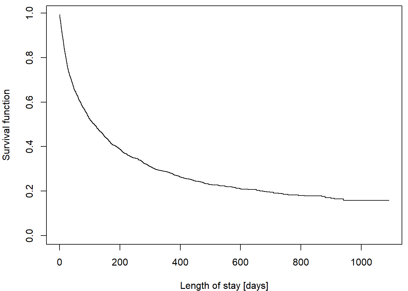
head=F, skip=14, col.names = c("los", "age", "rx", "gender", "married", "health", "censor"))In this dataset, length of stay (los) can be considered
continuous enough so that classical Kaplan-Meier estimator looks fairly
smooth:
We wish to demonstrate the use of the actuarial method. To do so,
consider the treated nursing home patients, with length of stay
(los) grouped into 100 day intervals:
nurshome$int = floor(nurshome$los/100)*100 # group in 100 day intervalsComparison of different approaches of estimation:
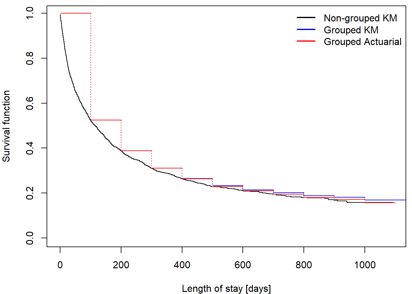
We can see that for low values of time there is merely any difference since \(r_j'\) and \(\overline{Y}(t_j)\) are large values with almost no impact on ratios used for estimation. However, there seems to emerge some difference for high values of time, since the negligible differences have accumulated and the actuarial update of ratios begins to notably lower the estimating ratios.
Estimation of hazard function
This grouped data approach enables us to estimate the hazard
functions using formulae in the section above. The resulting estimate
can be found in hazard output of lifetab
function.
We will not dive deep into the theory, but there is also a method for
obtaining smoothed estimator of hazard function using
library(muhaz). Check that these methods provide similar
results:
library(muhaz)
haz = muhaz(nurshome$los, nurshome$censor==0)
plot(haz)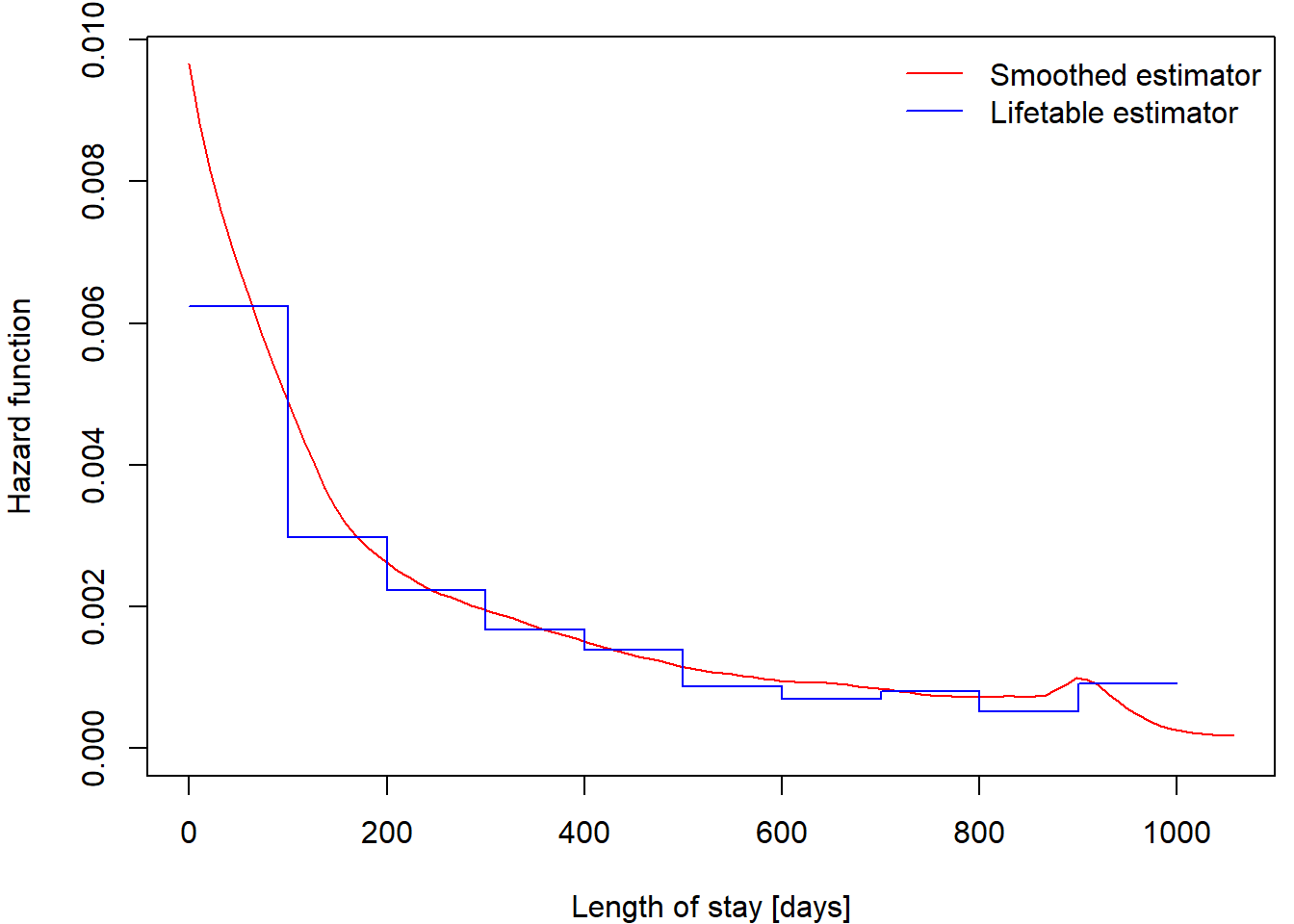
Based on other covariates in nurshome dataset choose
some interesting two subpopulations.
- Perform non-grouped KM estimation, grouped KM estimation and also the actuarial estimation of survival function.
- Plot the estimates to compare subpopulations and also the methods and comment on it.
- Estimate, plot and compare the hazard functions.
Advice: You can utilize plotting functions from previous exercise.
Mortality in the Czech Republic in 2021
Download dataset mort.RData.
There are three dataframes mort.m, mort.f and
mort containing mortality data from the Czech Republic in
the year 2021 for males, females and both genders combined. Each
dataframe has three columns:
iis an age group (going from the age \(i\) years to \(i+1\) years),Diis the number of deaths in the \(i\)-th age group in 2021,Yiis the number of people alive when they reached the age \(i\) (all at risk in \(i\)-th age group).
Think properly about the structure of this dataset. Does it follow the same structure as supposed in previous Exercise and the one supposed above? What does belonging to a certain age group mean?
If we blindly use lifetab function we obtain:
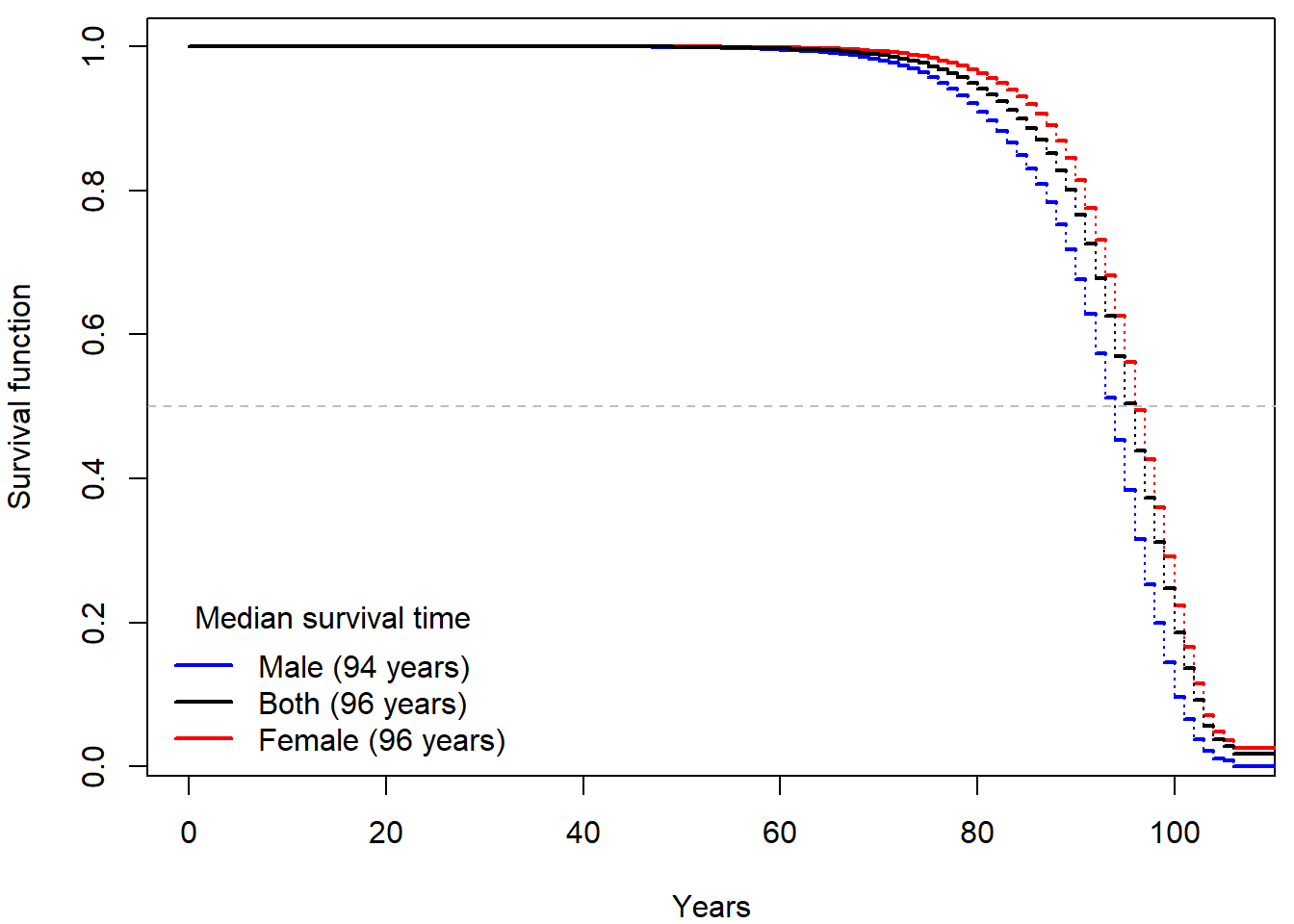
Inspired by the actuarial approach we base the estimate on
r_j = Yi -(Yi-Di)/2 and obtain the following estimate,
which inappropriately shortens the life span:
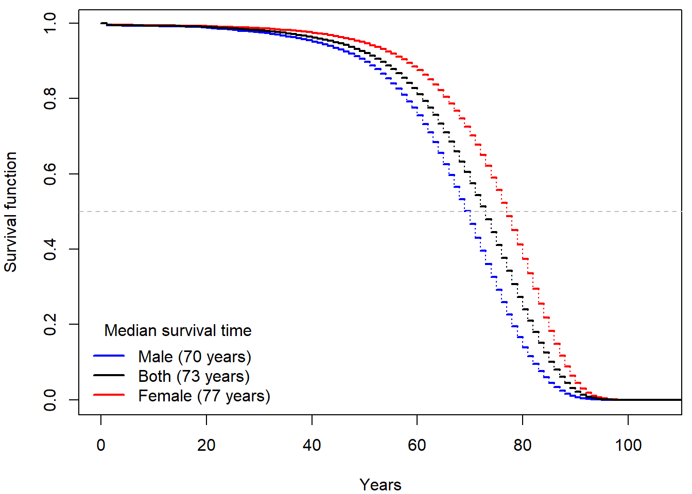
What would happen if we used simply 1 - Di/Yi for
estimation of survival of \(i\)-th age
group?
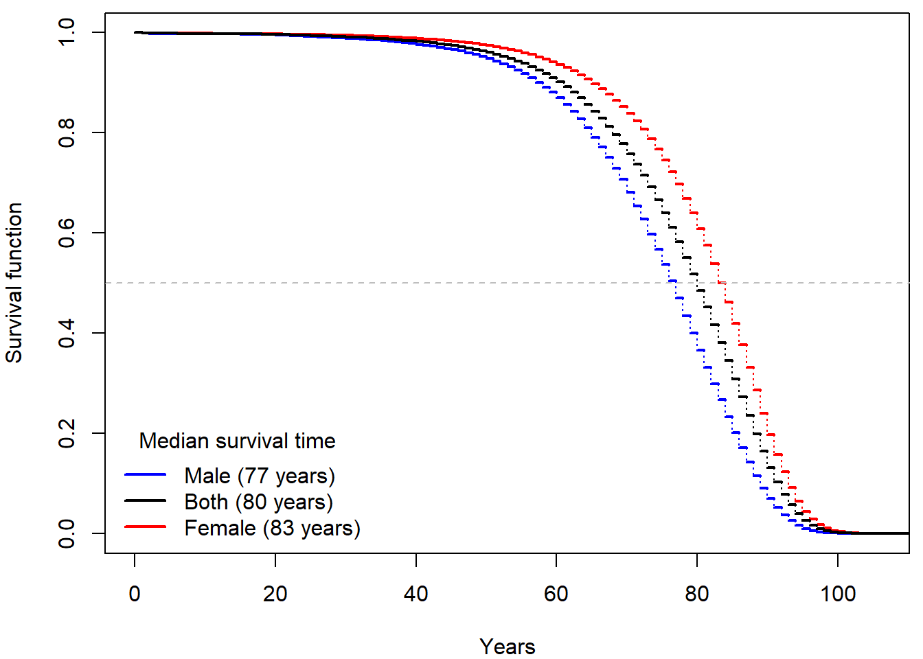
Try to reproduce the plots above. Why does lifetab
function give such non-senses? Can you try to explain it? What would be
the correct approach and why?
Compare (using suitable plots) your results to the official mortality tables created by ČSÚ: here for the males, here for the females. Can you recognize the columns in their table? Are their results comparable to yours?
If interested, examine the official guidelines (in Czech) of ČSÚ and see how the estimates could be further improved.
Include the (important) code, output and comments in your report.
- Deadline for report: Monday 28th November 9:00
Historical evolution of survival probability in the state territory of the Czech Republic
Official estimates of the survival function given by ČSÚ in 1920-2021: