The choice of two-sample test statistic
Jan Vávra
Exercise 6 (5th December 2022)
To succesfully complete the following task use the following shiny app.
Use this shiny app to fill the following table with the symbols:
- 1 = good choice,
- 2 = not good, not bad choice,
- 3 = inappropriate choice,
- ? = no idea.
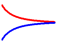
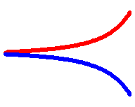
This symbol will represent your opinion on the choice of this particular two-sample statistic in the case of violation null hypothesis described by the plot of hazard functions.
Using the app find at least one example (distributions of survival times \(T_1\), \(T_2\) and their censoring distributions) where some choice of weight function is inappropriate (low power under evident H0 violation) while some other weight function rejects obvious violation of null hypothesis.
| Statistic | Weight function | \(G(\rho, \gamma)\) |  |
 |
 |
 |
 |
 |
|
|---|---|---|---|---|---|---|---|---|---|
| Logrank (Mantel) | \(1\) | \(G(0,0)\) | |||||||
| Prentice-Wilcoxon | \(\widehat{S}(t-)\) | \(G(1,0)\) | |||||||
| — | \(\left[1-\widehat{S}(t-)\right]\) | \(G(0, 1)\) | |||||||
| Fleming-Harrington | \(\rho = \gamma = 1\) | \(G(1, 1)\) |
The rest of this exercise is focused on real data analyses with different hazard shapes.
Compare survival distributions between the two groups of interest in the following datasets. Conduct the analysis according to the same steps as in the previous exercise.
Calculate and plot survival function.
Calculate and plot Nelson-Aalen estimators of cumulative hazard function.
Plot smoothed hazard functions.
Perform logrank, Prentice-Wilcoxon, \(G(0,1)\) or some particular \(G(\rho,\gamma)\) tests using functions
survdifforFHtestrcc. Interpret the results. Discuss the choice of weight function with respect to the power of the resulting test.
Since combining Exercises 5+6 could be time-consuming for you to do in one week, choose only 2 of the following 4 tasks to be solve together with homework from Exercise 5!
Activate the dataset veteran by calling
data(veteran). It includes 137 observations and eight
variables. The observations are lung cancer patients. The variable
time contains survival time (in days) since the start of
treatment. The variable status includes the event indicator
(1 = death, 0 = censoring). The variable trt distinguishes
two different treatments (1 = standard, 2 = experimental). The treatment
was randomly assigned to the patients.
Compare survival distributions between standard and experimental treatments.
Compare survival distributions between patients with Karnofsky scores up to 60 and over 60 (regardless of treatment assignment). These scores are stored in variable
karno.
Return to Exercise 3 Task 1, the nurshome dataset.
Perform the comparison of survival distributions of subpopulations of
your choice. Try to find some interesting division.
You should also be able to perform some simulation study for yourself:
Generate \(n_1=100\) censored observations from the Weibull distribution with shape parameter \(\alpha=0.7\) and scale parameter \(1/\lambda=2\). Its expectation is \(\Gamma(1+1/\alpha)/\lambda=2\Gamma(17/7)\doteq 2.53\).
Generate another sample of \(n_2=100\) censored observations from the exponential distribution with the same mean.
Let the censoring distribution in both samples be exponential with the rate \(\lambda=0.2\) (the expectation is \(1/\lambda=5\)), independent of survival. Put both samples in a single dataframe, introducing a variable distinguishing which sample each observation comes from.
Compare survival distributions between the two groups using the generated data. Conduct the analysis according to the steps 1–4 and display the true survival and hazard functions in the plots generated at steps 1–3 of the analysis.
- Deadline Ex5 (all of it) + Ex6 (task1 + just two of the tasks 2-5) : Tuesday 13th December 9:00