Generalizations of the Cox model
Jan Vávra
Bonus Exercise (not scheduled)
Cox proportional hazards model with time-invariant covariates
We observe \(n\) independent triplets \((X_i, \delta_i, \mathbf{Z}_i), i = 1, \ldots, n\), where
- \(X_i = \min \{T_i, C_i\}\) is censored failure time,
- \(\delta_i = \mathbb{I}_{(T_i \leq C_i)}\) is failure indicator,
- \(\mathbf{Z}_i\) is a vector of covariates.
We suppose that the hazard function \(\lambda\) of failure time distribution (assumed to be continuous) given covariates \(T|\mathbf{Z}\) is of the form: \[\lambda(t| \mathbf{Z}) = \lambda_0(t) \exp \left\{ \mathbf{Z}^\top \boldsymbol{\beta}\right\},\] where:
- \(\lambda_0(t)\) is the baseline hazard function,
- \(\boldsymbol{\beta} \in \mathbb{R}^p\) is unknown vector of regression coefficients.
See help(coxph) to discover all possibilities of this
function.
1) Stratification
Let us have a categorical covariate \(V\) which breaks the proportional hazards assumption so that the Cox model based inference is no longer valid. Dividing the data according to the level of \(V\) we create strata each of which has its own baseline hazard function \(\lambda_{0,j}\): \[ \lambda(t | \mathbf{Z}, V = j) = \lambda_{0, j}(t) \exp \left\{ \mathbf{Z}^\top \boldsymbol{\beta} \right\}. \] Hence, the proportional hazard assumption has been softened to hold only within each stratum but not between different strata: \[ \dfrac{\lambda(t | \mathbf{Z} + \mathbf{e_l}, V = j) }{\lambda(t | \mathbf{Z}, V = j) } = \dfrac{\lambda_{0, j}(t) \exp \left\{ \mathbf{Z}^\top \boldsymbol{\beta} + \beta_l \right\}}{\lambda_{0, j}(t) \exp \left\{ \mathbf{Z}^\top \boldsymbol{\beta} \right\}} = \exp \left\{ \beta_l \right\} \qquad \text{and} \qquad \dfrac{\lambda(t | \mathbf{Z}, V = j_1) }{\lambda(t | \mathbf{Z}, V = j_2) } = \dfrac{\lambda_{0, j_1}(t)}{\lambda_{0, j_2}(t)} \neq \text{const. for }\; j_1 \neq j_2. \]
If you want to include some stratification in your Cox model just
wrap the covariate by strata() inside the model
formula.
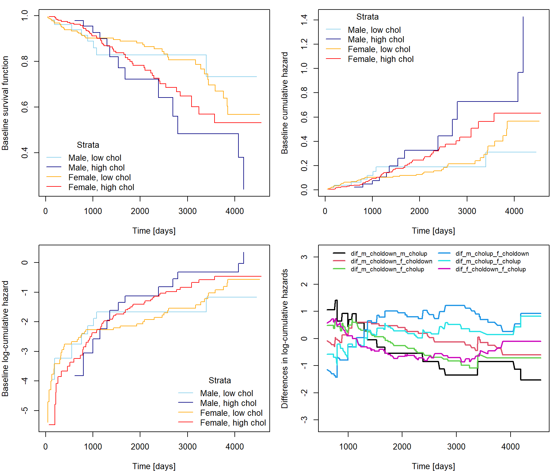
fit <- coxph(Surv(time,delta) ~ log(age) + hepato + strata(sex) + strata(chol>300), data=pbc)
cumhaz <- basehaz(fit)
# now contains 3 columns: cumhazard, time and stratification according to selected factor variable
Function basehaz extracts the baseline cumulative
hazards specific to each stratum (with centered other
covariates as default) that follow an obvious extension of Breslow
estimator: \[
\widehat{\Lambda}_{0,j} (t) = \int \limits_0^{t} \dfrac{\mathrm{d}
\overline{N}_j(s)}{\sum \limits_{i=1}^{n_j} Y_{j,i}(s) \exp \left\{
\widehat{\boldsymbol{\beta}}^\top \mathbf{Z}_{j,i}(s) \right\}}.
\] Survival and hazard curves for a certain patient then follow
the shape specific for the stratum to which the patient belongs.
library(survminer)
library(ggplot2)

newdata <- with(pbc, data.frame(age =    c(50),
                                hepato = c(0.5176056),
                                chol =   c(300),
                                sex =    "f"))
fitnew <- survfit(fit, newdata = newdata, conf.type = "plain")

# still produces all 4 possibilities even when chol and sex are given...
ggsurvplot(fitnew, data = newdata,
           conf.int = TRUE, censor= FALSE,
           ggtheme = theme_minimal())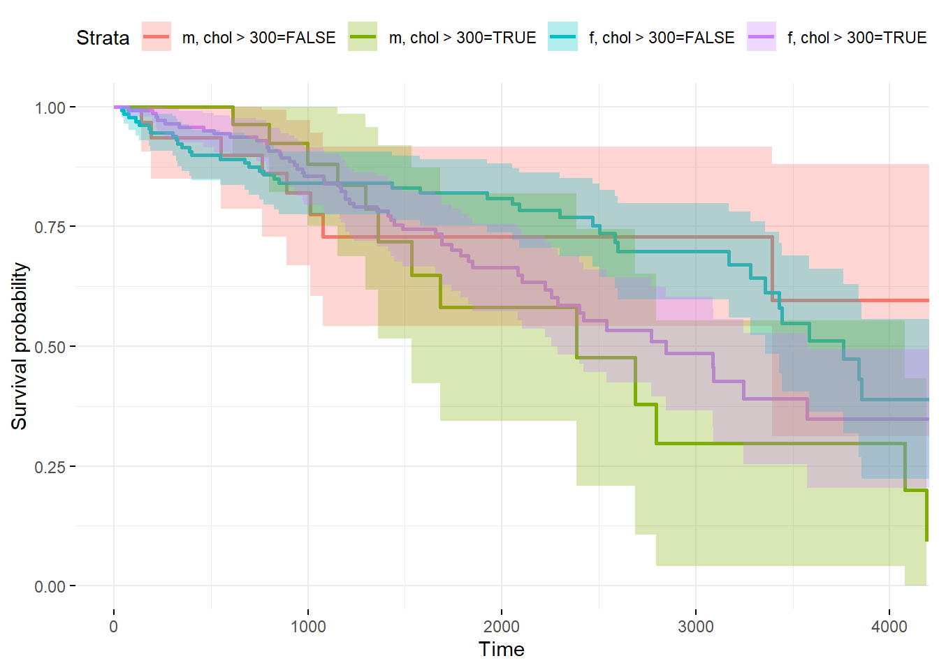
2) Semiparametric Regression for the Mean and Rate Functions of Recurrent Events - Lin et al. (2000)
Theory
See blackboard notes for more details.
We extend the concept of right censoring for the possibility of recurring events of one individual:
- 0 events: censoring time \(C\) is observed first (times of possible event are after \(C\), hence unobserved),
- 1 event: first observed event at \(T_1\) , then censoring time \(C > T_1\) hides all other possible events,
- \(\vdots\)
- \(k\) events: \(T_1 < T_2 < \cdots < T_k\) are observed event times before censoring time \(C > T_k\) happens.
Uncensored counting process \(N^\star(t)\) counts the number of events that occur in interval \([0,t]\). However, only his censored version \(N(t) = N^\star (t \wedge C)\) is observed. Also a \(p\)-dimensional covariate process \(\mathbf{Z}(t)\) is observed. Anderson and Gill model the intensity by \[ \lambda(t | \mathbf{Z}) = \lambda_0(t) \exp \left\{ \mathbf{Z}(t)^\top \boldsymbol{\beta} \right\}, \] where \(\lambda_0(\cdot)\) is unspecified baseline hazard function and \(\boldsymbol{\beta}_0\) is unknown vector of coefficients. Under this model, \(N^\star(t)\) is a time-transformed Poisson process in that \(N^\star (\Lambda^{-1}(t|\boldsymbol{Z}))\) is a Poisson process, where \(\Lambda^{-1}(t|\boldsymbol{Z})\) is the inverse function of \[ \Lambda(t|\boldsymbol{Z}) = \int \limits_0^t \exp \left\{ \mathbf{Z}(u)^\top \boldsymbol{\beta}\right\} \lambda_0(u) \,\mathrm{d} u. \] If \(\mathbf{Z}\) is time-invariant, then \(N^\star(t)\) is a non-homogeneous Poisson process.
Moreover, suppose that some subjects are more prone to recurrent events than others and that this heterogeneity can be characterized through the random-effect intensity model \[ \lambda(t | \mathbf{Z}) = \lambda_0(t) \; \eta \; \exp \left\{ \mathbf{Z}(t)^\top \boldsymbol{\beta} \right\}, \] where \(\eta\) is an unobserved unit-mean positive random variable that is independent of \(\mathbf{Z}\).
The estimator \(\widehat{\boldsymbol{\beta}}\) for \(\boldsymbol{\beta}_0\) can be found via partial likelihood as a solution of \[ \mathbf{U}_n(\boldsymbol{\beta}, t) = \sum \limits_{i=1}^n \int \limits_0^t \left[ \mathbf{Z}_i(u) - \overline{\mathbf{Z}}_n (\boldsymbol{\beta}, u) \right] \, \mathrm{d} N_i(u) = \sum \limits_{i=1}^n \sum \limits_{j=1}^{n_i} \left[ \mathbf{Z}_i(T_{i,j}) - \overline{\mathbf{Z}}_n (\boldsymbol{\beta}, T_{i,j}) \right] \overset{!}{=} \mathbf{0}. \] When no random-effects are present, asymptotic distribution for \(\mathbf{U}\) and \(\widehat{\boldsymbol{\beta}}\) can be (under some regularity conditions) found via martingale central limit theorem: \[ \frac{1}{\sqrt{n}} \mathbf{U}_n(\boldsymbol{\beta}_0, \tau) \underset{n \to \infty}{\overset{\mathcal{D}}{\longrightarrow}} N(\mathbf{0}, A) \qquad \text{and} \qquad \sqrt{n} \left( \widehat{\boldsymbol{\beta}} - \boldsymbol{\beta}_0\right)\underset{n \to \infty}{\overset{\mathcal{D}}{\longrightarrow}} N(\mathbf{0}, A^{-1}), \] where \[ A \equiv \mathsf{E}\, \left[ \int \limits_{0}^\tau \left( \mathbf{Z}_1(u) - \overline{\mathbf{z}} (\boldsymbol{\beta}_0, u) \right) \left( \mathbf{Z}_1(u) - \overline{\mathbf{z}} (\boldsymbol{\beta}_0, u) \right)^\top Y(u) \exp \left\{ \mathbf{Z}_1(u)^\top \boldsymbol{\beta} \right\} \, \mathrm{d} \Lambda_0(u) \right] . \]
However, under model with hidden heterogeneity we can no longer rely on martingale CLT, since \(M_i(t) = N_i(t) - \int_0^t Y_i(u) \exp \left\{ \mathbf{Z}(u)^\top \boldsymbol{\beta}_0\right\} \, \mathrm{d} \Lambda_0(u)\) are no longer martingales. Nevertheless, \(M_i\) can still replace \(N_i\) within the definition of scores. We will apply a different approach resembling the use of GEE with an independence working assumption for longitudinal data. Since \(\widehat{\boldsymbol{\beta}}\) is defined to be a Z-estimator we can divide \(\mathbf{U}_n(\boldsymbol{\beta}_0, t)\) into \[ \sum \limits_{i=1}^n \int \limits_0^t \left[ \mathbf{Z}_i(u) - \overline{\mathbf{z}} (\boldsymbol{\beta}_0, u) \right] \, \mathrm{d} M_i(u) + \sum \limits_{i=1}^n \int \limits_0^t \left[ \overline{\mathbf{z}} (\boldsymbol{\beta}_0, u) - \overline{\mathbf{Z}}_n (\boldsymbol{\beta}_0, u) \right] \, \mathrm{d} M_i(u), \] where for the first part we can apply iid CLT (as for Z-estimators) and show that second part is \(o_p(\sqrt{n})\). This yields asymptotic distribution of \(\frac{1}{\sqrt{n}} \mathbf{U}_n(\boldsymbol{\beta}_0, \tau)\) which can be transferred to convergence of \(\sqrt{n} \left( \widehat{\boldsymbol{\beta}} - \boldsymbol{\beta}_0\right)\) by Taylor expansion. Then we can apply modern empirical process theory to provide even weak convergence of processes. In the end we obtain \[ \frac{1}{\sqrt{n}} \mathbf{U}_n(\boldsymbol{\beta}_0, \tau) \underset{n \to \infty}{\overset{\mathcal{D}}{\longrightarrow}} N(\mathbf{0}, \Sigma) \qquad \text{and} \qquad \sqrt{n} \left( \widehat{\boldsymbol{\beta}} - \boldsymbol{\beta}_0\right)\underset{n \to \infty}{\overset{\mathcal{D}}{\longrightarrow}} N(\mathbf{0}, A^{-1}\Sigma A^{-1}), \]
where \[ \Sigma = \Sigma(\tau, \tau) \quad \text{and} \quad \Sigma(s,t) = \mathsf{E}\, \left[ \int \limits_{0}^s \left( \mathbf{Z}_1(u) - \overline{\mathbf{z}} (\boldsymbol{\beta}_0, u) \right) \, \mathrm{d} M_1(u) \int \limits_{0}^t \left( \mathbf{Z}_1(v) - \overline{\mathbf{z}} (\boldsymbol{\beta}_0, v) \right)^\top \, \mathrm{d} M_1(v) \right] \] is the covariance function of limitting process to which \(\frac{1}{\sqrt{n}} \mathbf{U}_n(\boldsymbol{\beta}_0, t)\) weakly converges.
In general \(\Sigma \neq A\) and hence the correct asymptotic variance of \(\widehat{\boldsymbol{\beta}}\) is not \(A^{-1}\), but rather \(\Gamma = A^{-1} \Sigma A^{-1}\). We can estimate the quantities by: \[ \begin{align} \widehat{A} &= \frac{1}{n} \sum \limits_{i=1}^n \left[ \int \limits_{0}^\tau \left( \mathbf{Z}_i(u) - \overline{\mathbf{Z}}_n (\widehat{\boldsymbol{\beta}}, u) \right) \left( \mathbf{Z}_i(u) - \overline{\mathbf{Z}}_n (\widehat{\boldsymbol{\beta}}, u) \right)^\top Y_i(u) \exp \left\{ \mathbf{Z}_i(u)^\top \widehat{\boldsymbol{\beta}} \right\} \, \dfrac{ \mathrm{d} \overline{N}(u) }{ n S^{(0)}(\widehat{\boldsymbol{\beta}}, u) } \right] \\ &= \frac{1}{n} \sum \limits_{i=1}^n \left[ \int \limits_{0}^\tau \left[ \dfrac{S^{(2)}(\widehat{\boldsymbol{\beta}}, u)}{S^{(0)}(\widehat{\boldsymbol{\beta}}, u)} - \overline{\mathbf{Z}}_n (\widehat{\boldsymbol{\beta}}, u) \overline{\mathbf{Z}}_n (\widehat{\boldsymbol{\beta}}, u)^\top \right] \, \mathrm{d} N_i(u) \right], \\ \widehat{\Sigma} &= \frac{1}{n} \sum \limits_{i=1}^n \left[ \int \limits_{0}^\tau \left( \mathbf{Z}_i(u) - \overline{\mathbf{Z}}_n (\widehat{\boldsymbol{\beta}}, u) \right) \, \mathrm{d} \widehat{M}_i(u) \int \limits_{0}^\tau \left( \mathbf{Z}_i(v) - \overline{\mathbf{Z}}_n (\widehat{\boldsymbol{\beta}}, v) \right)^\top \, \mathrm{d} \widehat{M}_i(v) \right], \\ \widehat{M}_i(t) &= N_i(t) - \int \limits_{0}^t Y_i(u) \exp \left\{ \mathbf{Z}_i(u)^\top \widehat{\boldsymbol{\beta}}\right\} \dfrac{ \mathrm{d} \overline{N}(u) }{ n S^{(0)}(\widehat{\boldsymbol{\beta}}, u) }. \end{align} \] We shall refer to \(\widehat{\Gamma}\) and \(\widehat{A}^{-1}\) as the robust and naive covariance matrix estimators respectively.
Recurring events and robust variance estimator in R
How do we tell coxph function that there are potentially
multiple events per patient? The data has to be passed to
coxph in a very special format, similar to the one used for
time-varying covariates (see Exercise 8). We
need to create intervals (start, stop) at the end of which
an event is observed with the exception of the last interval, where the
patient is censored.
| Patient id | enum | start | stop | event |
|---|---|---|---|---|
| id | \(1\) | \(0\) | \(T_1\) | \(1\) |
| id | \(2\) | \(T_1\) | \(T_2\) | \(1\) |
| id | \(3\) | \(T_2\) | \(T_3\) | \(1\) |
| id | \(\vdots\) | \(\vdots\) | \(\vdots\) | \(1\) |
| id | \(k\) | \(T_{k-1}\) | \(T_k\) | \(1\) |
| id | \(k+1\) | \(T_k\) | \(C\) | \(0\) |
The last row can be missing if \(T_k = C\), that is, the last time we checked the patient is also the last time he experienced an event.
Data are passed to coxph function by the following
way
coxph(Surv(start, stop, event)~ formula, data)This, however, works with the naive variance estimator. If hidden heterogeneity on patient level is to be expected, then the robust variance estimator should be used:
coxph(Surv(start, stop, event)~ formula, data, cluster = id)
# or
coxph(Surv(start, stop, event)~ formula + cluster(id), data)
However, we can use the robust variance estimator in the case of standard Cox model (without recurring events) if we suspect that some assumptions (proportionality of hazards) are violated, compare
summary(coxph(Surv(time,delta)~ log(age) + chol + hepato, data=pbc))
summary(coxph(Surv(time,delta)~ log(age) + chol + hepato, data=pbc, robust = T))
Simulation study
Let us have \(n \in \{ 100, 200, 500 \}\) patients, half having covariate \(Z = 0\) and the other half \(Z = 1\). Let us set:
- \(\lambda_0(t) = 1\),
- \(\beta_0 = 0.5\),
- \(\eta \sim \Gamma\left(\sigma^{-2},\; \sigma^2\right)\) so that \(\mathsf{E}\, \eta = 1\) and \(\mathsf{var}\, \eta = \sigma^2 \in \{ 0, 0.25, 0.5, 1 \}\),
- \(\lambda(t | Z) = \lambda_0(t)\, \eta\, \exp\{\beta_0 Z\}\),
- assume recurred events model and set censoring time \(C = 3\),
- create \(M = 1000\) datasets.
For each simulated dataset, we estimated \(\beta_0\) under two different intensity models:
- \(\lambda(t | Z) = \lambda_0(t)\, \exp\{\beta_0 Z\}\),
- \(\lambda(t | Z) = \lambda_0(t)\, \exp\{\beta_0 Z + \gamma_0 X(t)\}\),
where \(X(t)\) is a time-varying covariate indicating occurance of event in previous unit of time: \[ X(t) \left\{ \begin{aligned} 1, &\qquad \text{if there was an event within the interval }\; [t -1,\, t), \\ 0, &\qquad \text{otherwise}. \end{aligned} \right. \] We also estimate the variance by both naive and robust estimators.
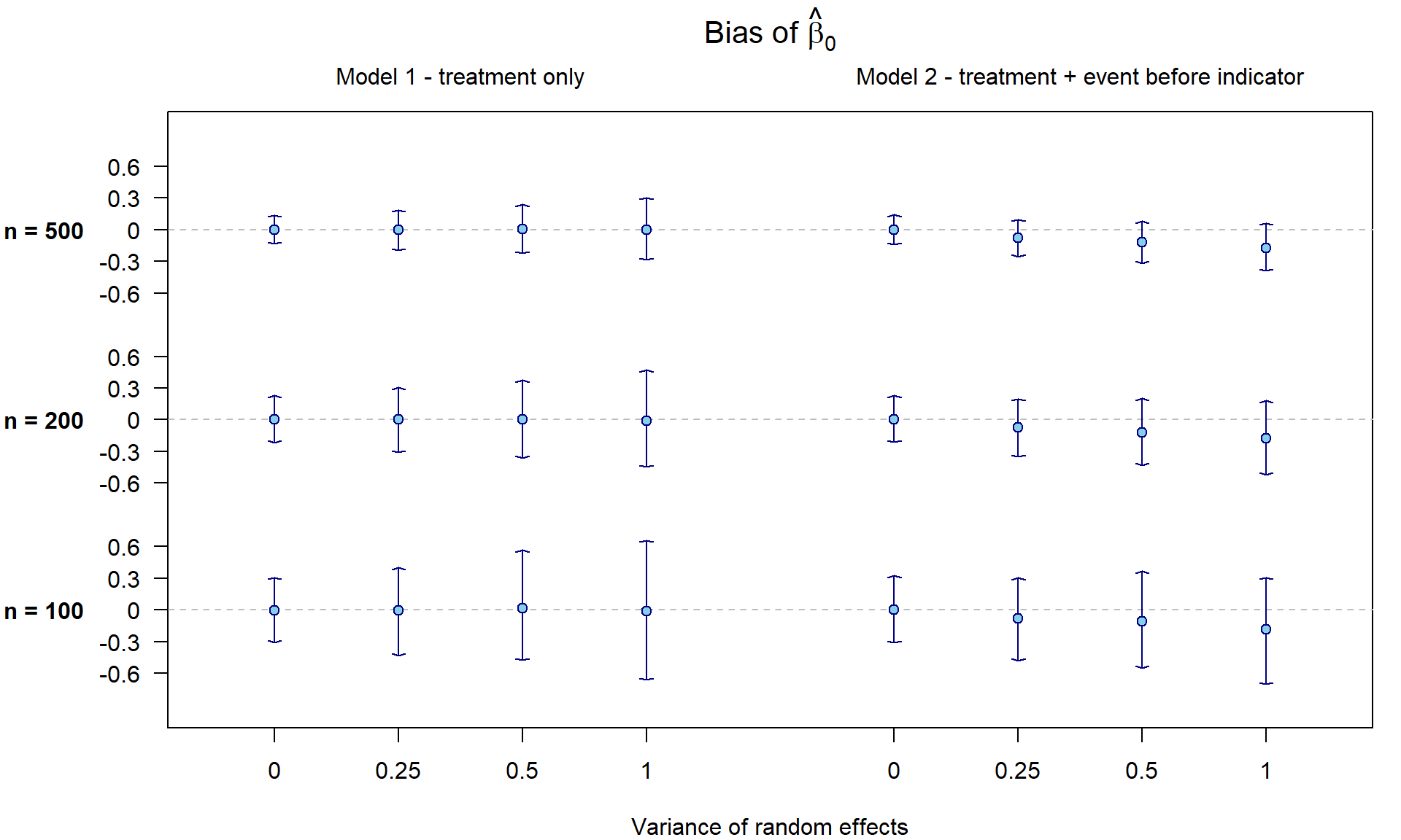
Let us first check whether the point estimator \(\widehat{\beta}_0\) is unbiased in
all considered settings by plotting the mean and 0.025 and 0.975
quantiles of \(M\) simulated \(\widehat{\beta}_0 - \beta_0\). Under model
1 the estimate of \(\beta_0\) is
unbiased. However, under model 2 the estimator of \(\beta_0\) is biased downwards unless \(\sigma^2 = 0\).
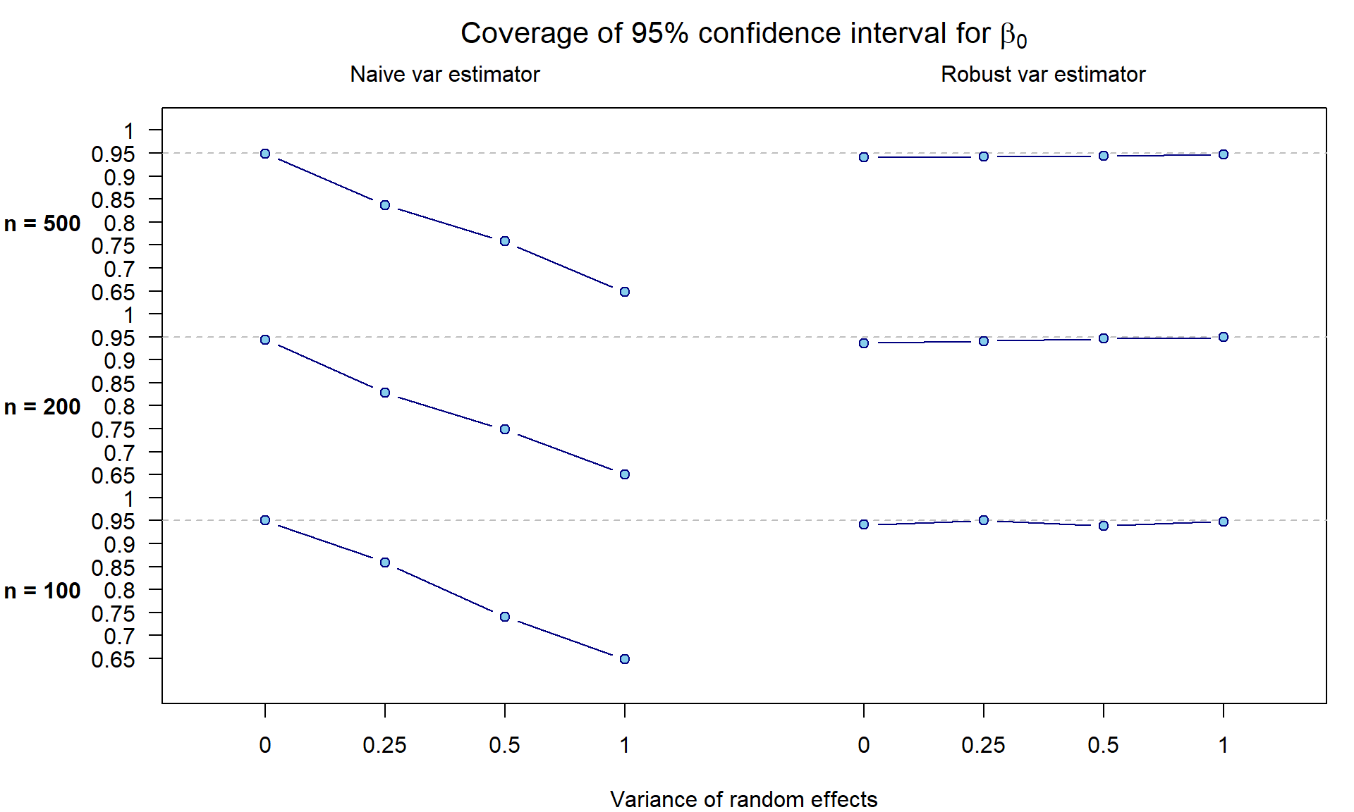
Under model 1, we have also constructed \(M\) confidence intervals for \(\beta_0\) with the use of naive
and robust variance estimators while being interested whether
the coverage corresponds to the used 0.95. Apparently, the
naive variance estimator cannot handle the hidden heterogeneity
caused by random effects \(\eta\):
Real data analysis - CGD study
We now apply the methods proposed to the multiple-infection data taken from the CGD study presented by Fleming and Harrington (1991), section 4.4. CGD is a group of inherited rare disorders of the immune function characterized by recurrent pyogenic infections.
library(survival)
data(cgd)
#help(cgd)
cgd[cgd$id==109,"height"] <- 100 + cgd[cgd$id==109,"height"] # probably forgotten digit?
head(cgd[,c(1:6, 13:16)], 13)
## id center random treat sex age tstart enum tstop status
## 1 1 Scripps Institute 1989-06-07 rIFN-g female 12 0 1 219 1
## 2 1 Scripps Institute 1989-06-07 rIFN-g female 12 219 2 373 1
## 3 1 Scripps Institute 1989-06-07 rIFN-g female 12 373 3 414 0
## 4 2 Scripps Institute 1989-06-07 placebo male 15 0 1 8 1
## 5 2 Scripps Institute 1989-06-07 placebo male 15 8 2 26 1
## 6 2 Scripps Institute 1989-06-07 placebo male 15 26 3 152 1
## 7 2 Scripps Institute 1989-06-07 placebo male 15 152 4 241 1
## 8 2 Scripps Institute 1989-06-07 placebo male 15 241 5 249 1
## 9 2 Scripps Institute 1989-06-07 placebo male 15 249 6 322 1
## 10 2 Scripps Institute 1989-06-07 placebo male 15 322 7 350 1
## 11 2 Scripps Institute 1989-06-07 placebo male 15 350 8 439 0
## 12 3 Scripps Institute 1989-06-08 rIFN-g male 19 0 1 382 0
## 13 4 Scripps Institute 1989-06-23 rIFN-g male 12 0 1 388 0To evaluate the ability of gamma interferon in reducing the rate of infection, a placebo- controlled randomized clinical trial was conducted between October 1988 and March 1989. A total of 128 patients were enrolled into the study. By the end of the trial, 14 of 63 treated patients and 30 of 65 untreated patients had experienced at least one infection. Of the 30 untreated patients with at least one infection, five had experienced two infections, four others had experienced three and three patients had four or more. Of the 14 treated patients with at least one infection, four experienced two and another had a third infection.
table(table(cgd$id)-1, cgd$treat[cgd$enum==1])##
## placebo rIFN-g
## 0 35 49
## 1 19 9
## 2 4 4
## 3 4 1
## 4 1 0
## 5 1 0
## 7 1 0Available covariates:
treat= treatment: placebo or gamma interferon,sex= gender: male or femaleinherit= pattern of inheritancesteroids= use of steroids at study entry, 1=yespropylac= use of prophylactic antibiotics at study entryhos.cat= a categorization of the centers into 4 groupsage= age in years, at study entryheight= height in cm at study entryweight= weight in kg at study entry
summary(cgd[cgd$enum==1, catregs])## treat sex inherit fsteroids fpropylac hos.cat
## placebo:65 male :104 X-linked :86 No :125 No : 17 US:NIH :26
## rIFN-g :63 female: 24 autosomal:42 Yes: 3 Yes:111 US:other :63
## Europe:Amsterdam:19
## Europe:other :20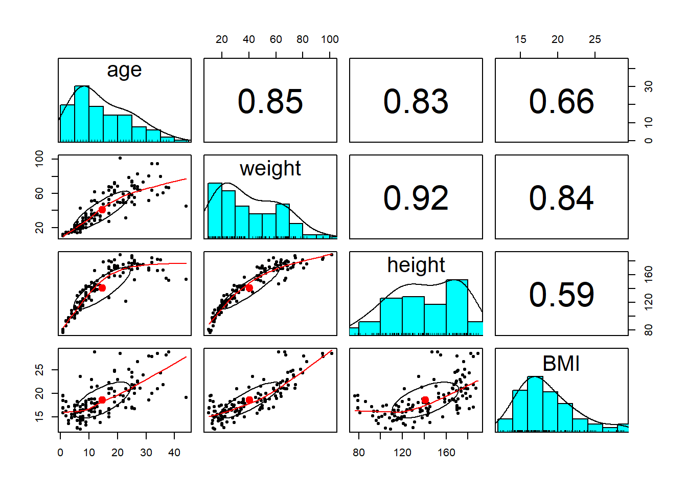
Let us first do the exploratory analysis.
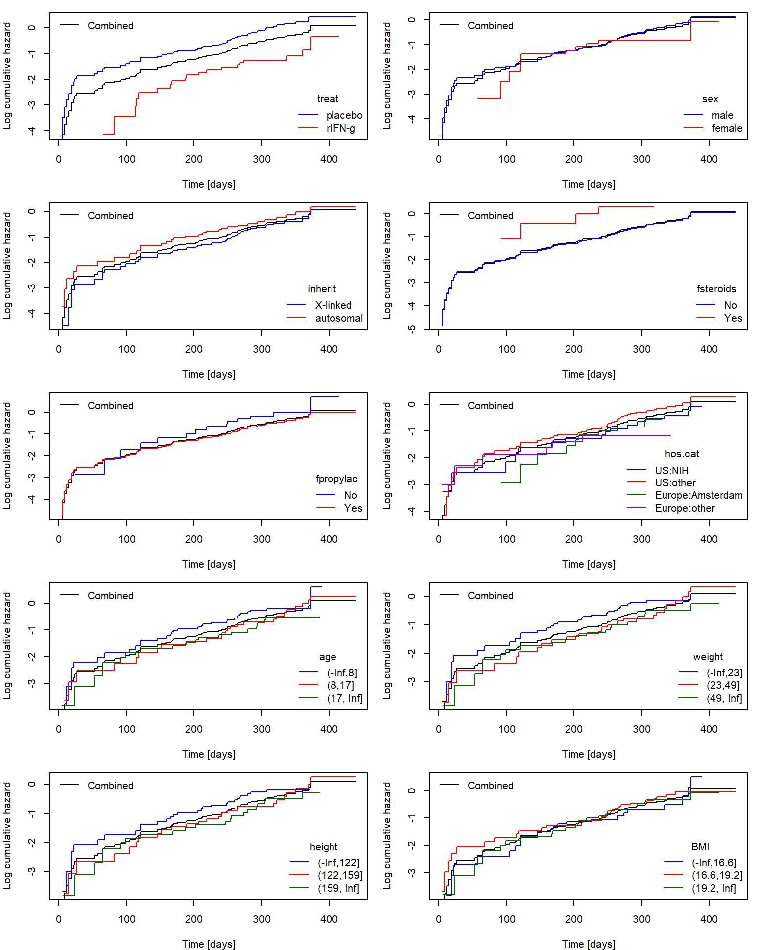
Fit coxph model with both naive and
robust estimator to see how it impacts the significance of
coefficients. We also confirm that beside the treatment, other
covariates seem not to have strong influence on the hazard (maybe with
the exception of age and inherit).
formula <- as.formula(paste0("Surv(tstart, tstop, status) ~ ",
                      paste0(c(catregs, numregs), collapse = "+")))
fit0n <- coxph(formula, cgd)
summary(fit0n)
## Call:
## coxph(formula = formula, data = cgd)
##
## n= 203, number of events= 76
##
## coef exp(coef) se(coef) z Pr(>|z|)
## treatrIFN-g -1.1862901 0.3053520 0.2836876 -4.182 2.89e-05 ***
## sexfemale -0.7631382 0.4662011 0.3945553 -1.934 0.05309 .
## inheritautosomal 0.7367987 2.0892364 0.2988963 2.465 0.01370 *
## fsteroidsYes 1.9096973 6.7510448 0.6197629 3.081 0.00206 **
## fpropylacYes -0.6297312 0.5327350 0.3563761 -1.767 0.07722 .
## hos.catUS:other 0.0007824 1.0007827 0.3339982 0.002 0.99813
## hos.catEurope:Amsterdam -0.7899998 0.4538449 0.5031301 -1.570 0.11638
## hos.catEurope:other -0.5750872 0.5626558 0.5032476 -1.143 0.25314
## age -0.0853151 0.9182229 0.0370461 -2.303 0.02128 *
## weight 0.0111020 1.0111638 0.0414518 0.268 0.78883
## height 0.0063190 1.0063390 0.0193619 0.326 0.74415
## BMI 0.0098092 1.0098575 0.1155471 0.085 0.93235
## ---
## Signif. codes: 0 '***' 0.001 '**' 0.01 '*' 0.05 '.' 0.1 ' ' 1
##
## exp(coef) exp(-coef) lower .95 upper .95
## treatrIFN-g 0.3054 3.2749 0.1751 0.5324
## sexfemale 0.4662 2.1450 0.2151 1.0102
## inheritautosomal 2.0892 0.4786 1.1630 3.7533
## fsteroidsYes 6.7510 0.1481 2.0037 22.7465
## fpropylacYes 0.5327 1.8771 0.2649 1.0712
## hos.catUS:other 1.0008 0.9992 0.5200 1.9259
## hos.catEurope:Amsterdam 0.4538 2.2034 0.1693 1.2167
## hos.catEurope:other 0.5627 1.7773 0.2098 1.5087
## age 0.9182 1.0891 0.8539 0.9874
## weight 1.0112 0.9890 0.9323 1.0967
## height 1.0063 0.9937 0.9689 1.0453
## BMI 1.0099 0.9902 0.8052 1.2665
##
## Concordance= 0.72 (se = 0.033 )
## Likelihood ratio test= 45.8 on 12 df, p=8e-06
## Wald test = 39.06 on 12 df, p=1e-04
## Score (logrank) test = 43.14 on 12 df, p=2e-05fit0r <- coxph(formula, cgd, cluster = id)
summary(fit0r)## Call:
## coxph(formula = formula, data = cgd, cluster = id)
##
## n= 203, number of events= 76
##
## coef exp(coef) se(coef) robust se z Pr(>|z|)
## treatrIFN-g -1.1862901 0.3053520 0.2836876 0.3345991 -3.545 0.000392 ***
## sexfemale -0.7631382 0.4662011 0.3945553 0.4551924 -1.677 0.093637 .
## inheritautosomal 0.7367987 2.0892364 0.2988963 0.3998735 1.843 0.065390 .
## fsteroidsYes 1.9096973 6.7510448 0.6197629 0.8743691 2.184 0.028956 *
## fpropylacYes -0.6297312 0.5327350 0.3563761 0.3534758 -1.782 0.074824 .
## hos.catUS:other 0.0007824 1.0007827 0.3339982 0.3525238 0.002 0.998229
## hos.catEurope:Amsterdam -0.7899998 0.4538449 0.5031301 0.4799475 -1.646 0.099761 .
## hos.catEurope:other -0.5750872 0.5626558 0.5032476 0.4989064 -1.153 0.249035
## age -0.0853151 0.9182229 0.0370461 0.0307644 -2.773 0.005551 **
## weight 0.0111020 1.0111638 0.0414518 0.0384167 0.289 0.772591
## height 0.0063190 1.0063390 0.0193619 0.0216979 0.291 0.770876
## BMI 0.0098092 1.0098575 0.1155471 0.1010265 0.097 0.922651
## ---
## Signif. codes: 0 '***' 0.001 '**' 0.01 '*' 0.05 '.' 0.1 ' ' 1
##
## exp(coef) exp(-coef) lower .95 upper .95
## treatrIFN-g 0.3054 3.2749 0.1585 0.5883
## sexfemale 0.4662 2.1450 0.1910 1.1377
## inheritautosomal 2.0892 0.4786 0.9541 4.5747
## fsteroidsYes 6.7510 0.1481 1.2165 37.4658
## fpropylacYes 0.5327 1.8771 0.2665 1.0651
## hos.catUS:other 1.0008 0.9992 0.5015 1.9971
## hos.catEurope:Amsterdam 0.4538 2.2034 0.1772 1.1626
## hos.catEurope:other 0.5627 1.7773 0.2116 1.4959
## age 0.9182 1.0891 0.8645 0.9753
## weight 1.0112 0.9890 0.9378 1.0902
## height 1.0063 0.9937 0.9644 1.0501
## BMI 1.0099 0.9902 0.8284 1.2310
##
## Concordance= 0.72 (se = 0.038 )
## Likelihood ratio test= 45.8 on 12 df, p=8e-06
## Wald test = 33.62 on 12 df, p=8e-04
## Score (logrank) test = 43.14 on 12 df, p=2e-05, Robust = 15.58 p=0.2
##
## (Note: the likelihood ratio and score tests assume independence of
## observations within a cluster, the Wald and robust score tests do not).Model with the treatment only (naive variance estimator):
fit1n <- coxph(Surv(tstart, tstop, status) ~ treat, cgd)
summary(fit1n)
## Call:
## coxph(formula = Surv(tstart, tstop, status) ~ treat, data = cgd)
##
## n= 203, number of events= 76
##
## coef exp(coef) se(coef) z Pr(>|z|)
## treatrIFN-g -1.0953 0.3344 0.2610 -4.196 2.71e-05 ***
## ---
## Signif. codes: 0 '***' 0.001 '**' 0.01 '*' 0.05 '.' 0.1 ' ' 1
##
## exp(coef) exp(-coef) lower .95 upper .95
## treatrIFN-g 0.3344 2.99 0.2005 0.5578
##
## Concordance= 0.629 (se = 0.029 )
## Likelihood ratio test= 20.11 on 1 df, p=7e-06
## Wald test = 17.61 on 1 df, p=3e-05
## Score (logrank) test = 19.42 on 1 df, p=1e-05Model with the treatment only (robust variance estimator):
fit1r <- coxph(Surv(tstart, tstop, status) ~ treat, cgd, cluster = id)
summary(fit1r)
## Call:
## coxph(formula = Surv(tstart, tstop, status) ~ treat, data = cgd,
## cluster = id)
##
## n= 203, number of events= 76
##
## coef exp(coef) se(coef) robust se z Pr(>|z|)
## treatrIFN-g -1.0953 0.3344 0.2610 0.3119 -3.511 0.000446 ***
## ---
## Signif. codes: 0 '***' 0.001 '**' 0.01 '*' 0.05 '.' 0.1 ' ' 1
##
## exp(coef) exp(-coef) lower .95 upper .95
## treatrIFN-g 0.3344 2.99 0.1815 0.6164
##
## Concordance= 0.629 (se = 0.032 )
## Likelihood ratio test= 20.11 on 1 df, p=7e-06
## Wald test = 12.33 on 1 df, p=4e-04
## Score (logrank) test = 19.42 on 1 df, p=1e-05, Robust = 10.19 p=0.001
##
## (Note: the likelihood ratio and score tests assume independence of
## observations within a cluster, the Wald and robust score tests do not).Model with indicator of whether an infection occured in past 60 days (covariate changing in time). We shall split the interval data where the time period between two events is higher than 60 days and fill it with event=0.
days <- 60
cgd$infected60 <- 0
newcgd <- data.frame()
for(id in unique(cgd$id)){
  datai <- cgd[cgd$id == id, ]
  cgdi <- datai[1,]
  j <- 1
  infend <- cgdi[1,"tstop"] + days
  while(j < dim(datai)[1]){
    j <- j+1
    if(infend < datai[j,"tstop"]){
      # other infection more than 60days after --> divide into two new rows
      new1 <- datai[j,]
      new1[1,c("tstop", "status", "infected60")] <- c(infend, 0, 1) # no event, just change of infected60
      new2 <- datai[j,]
      new2[1,c("tstart", "infected60")] <- c(infend, 0) # keep status, change of infected60
      cgdi <- rbind(cgdi, new1, new2)
    }else{
      # again infected (or censored) within 60days
      new1 <- datai[j,]
      new1[1,"infected60"] <- 1 # just change of infected60
      cgdi <- rbind(cgdi, new1)
    }
    # change the next end of infection
    if(datai[j,"status"]){
      infend <- datai[j,"tstop"] + days
    }
  }

  newcgd <- rbind(newcgd, cgdi)
}
newcgd[1:20, c("id","enum","treat","tstart","tstop","status","infected60")]
## id enum treat tstart tstop status infected60
## 1 1 1 rIFN-g 0 219 1 0
## 2 1 2 rIFN-g 219 279 0 1
## 21 1 2 rIFN-g 279 373 1 0
## 3 1 3 rIFN-g 373 414 0 1
## 4 2 1 placebo 0 8 1 0
## 5 2 2 placebo 8 26 1 1
## 6 2 3 placebo 26 86 0 1
## 61 2 3 placebo 86 152 1 0
## 7 2 4 placebo 152 212 0 1
## 71 2 4 placebo 212 241 1 0
## 8 2 5 placebo 241 249 1 1
## 9 2 6 placebo 249 309 0 1
## 91 2 6 placebo 309 322 1 0
## 10 2 7 placebo 322 350 1 1
## 11 2 8 placebo 350 410 0 1
## 111 2 8 placebo 410 439 0 0
## 12 3 1 rIFN-g 0 382 0 0
## 13 4 1 rIFN-g 0 388 0 0
## 14 5 1 placebo 0 246 1 0
## 15 5 2 placebo 246 253 1 1Inclusion of such infection indicator however reduces the effect of treatment by about 10%. This is consistent with the simulation results that the estimator of the treatment effect has a negative bias if there is overdispersion. Naive variance estimator now performs much better since some of the heterogeneity has been captured by the infection indicator (which used to be the solution before robust variance estimator was suggested):
fit2n <- coxph(Surv(tstart, tstop, status) ~ treat + infected60, newcgd)
summary(fit2n)
## Call:
## coxph(formula = Surv(tstart, tstop, status) ~ treat + infected60,
## data = newcgd)
##
## n= 244, number of events= 76
##
## coef exp(coef) se(coef) z Pr(>|z|)
## treatrIFN-g -0.9874 0.3726 0.2659 -3.713 0.000205 ***
## infected60 0.7122 2.0385 0.2933 2.428 0.015178 *
## ---
## Signif. codes: 0 '***' 0.001 '**' 0.01 '*' 0.05 '.' 0.1 ' ' 1
##
## exp(coef) exp(-coef) lower .95 upper .95
## treatrIFN-g 0.3726 2.6841 0.2212 0.6274
## infected60 2.0385 0.4906 1.1472 3.6222
##
## Concordance= 0.655 (se = 0.031 )
## Likelihood ratio test= 25.38 on 2 df, p=3e-06
## Wald test = 24.2 on 2 df, p=6e-06
## Score (logrank) test = 27.05 on 2 df, p=1e-06Robust variance estimator:
fit2r <- coxph(Surv(tstart, tstop, status) ~ treat + infected60, newcgd, cluster = id)
summary(fit2r)
## Call:
## coxph(formula = Surv(tstart, tstop, status) ~ treat + infected60,
## data = newcgd, cluster = id)
##
## n= 244, number of events= 76
##
## coef exp(coef) se(coef) robust se z Pr(>|z|)
## treatrIFN-g -0.9874 0.3726 0.2659 0.2947 -3.351 0.000807 ***
## infected60 0.7122 2.0385 0.2933 0.2544 2.799 0.005121 **
## ---
## Signif. codes: 0 '***' 0.001 '**' 0.01 '*' 0.05 '.' 0.1 ' ' 1
##
## exp(coef) exp(-coef) lower .95 upper .95
## treatrIFN-g 0.3726 2.6841 0.2091 0.6638
## infected60 2.0385 0.4906 1.2381 3.3564
##
## Concordance= 0.655 (se = 0.034 )
## Likelihood ratio test= 25.38 on 2 df, p=3e-06
## Wald test = 22.15 on 2 df, p=2e-05
## Score (logrank) test = 27.05 on 2 df, p=1e-06, Robust = 10.27 p=0.006
##
## (Note: the likelihood ratio and score tests assume independence of
## observations within a cluster, the Wald and robust score tests do not).