Confidence intervals and bands for survival function
Jan Vávra
Exercise 4 (28th November 2022)
Theory
The Kaplan-Meier [KM] estimator of the survival function is \[ \widehat{S}(t)=\prod_{\{i: t_i\leq t\}}\biggl[1-\frac{\Delta\overline{N}(t_i)}{\overline{Y}(t_i)}\biggr]. \] A uniformly consistent estimator of the variance of \(\sqrt{n}[\widehat{S}(t)-S(t)]\) is \[ \widehat{V}(t)=\widehat{S}^2(t)\widehat{\sigma}(t)= \widehat{S}^2(t)\int_0^t \frac{n \,\mathrm{d}\overline{N}(u)}{\overline{Y}(u)[\overline{Y}(u)-\Delta\overline{N}(u)]} = \widehat{S}^2(t) \cdot n \cdot \sum \limits_{\{j:t_j \leq t\}} \dfrac{\Delta \overline{N}(t_j)}{\overline{Y}(t_j)[\overline{Y}(t_j)-\Delta\overline{N}(t_j)]} \] (Greenwood formula).
An asymptotic pointwise \(100(1-\alpha)\)% confidence interval for \(S(t)\) at a fixed \(t\) is \[ \biggl( \widehat{S}(t)\Bigl[1-u_{1-\alpha/2}\sqrt{\widehat{\sigma}(t)/n}\Bigr],\, \widehat{S}(t)\Bigl[1+u_{1-\alpha/2}\sqrt{\widehat{\sigma}(t)/n}\Bigr] \biggr). \] Asymptotic simultaneous \(100(1-\alpha)\)% Hall-Wellner confidence bands for \(S(t)\) over \(t\in\langle 0,\tau\rangle\) (for some pre-specified \(\tau\)) are \[ \biggl( \widehat{S}(t)\Bigl\{1-k_{1-\alpha}(\widehat{K}(\tau))\bigl[1+\widehat{\sigma}(t)\bigr]/\sqrt{n}\Bigr\},\, \widehat{S}(t)\Bigl\{1+k_{1-\alpha}(\widehat{K}(\tau))\bigl[1+\widehat{\sigma}(t)\bigr]/\sqrt{n}\Bigr\} \biggr), \] where \(\widehat{K}(t)=\widehat{\sigma}(t)/[1+\widehat{\sigma}(t)]\) and \(k_{1-\alpha}(t)\), \(t\in(0,1\rangle\), satisfies the equation \[ \text{P}\bigl[\sup_{u\in\langle 0,t\rangle}|B(u)|>k_{1-\alpha}(t)\bigr]=\alpha, \] where \(B\) is the Brownian bridge.
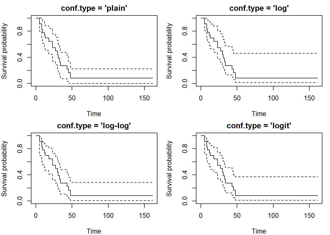
There are variations of confidence intervals and confidence bounds for \(S(t)\) based on various transformations (\(\log\), \(\log(-\log)\), \(\arcsin\), …). Formulae for these intervals can be derived by the delta method.
The use of the delta-method: pointwise CI.
Implementation in R
Pointwise confidence intervals
The function survfit in the library
survival calculates pointwise confidence intervals. The
argument conf.type specifies the transformation
(conf.type="plain" means no transformation), the argument
conf.int specifies the coverage probability (default 0.95).
Be careful, the default value is conf.type="log"!
Regardless of selected conf.type, variable
std.err always refers to \(\sqrt{
\widehat{\sigma}(t)/n}\), which can be computed as follows:
se <- sqrt(cumsum(fit$n.event/(fit$n.risk*(fit$n.risk-fit$n.event))))
summary(fit$std.err - se)
Confidence intervals are stored in the output object of the function
survfit, the components are called upper and
lower. The contents of survfit objects can be
also displayed by the function summary.
The function plot called on survfit objects
plots the confidence intervals included in the input object. The
argument conf.int determines whether or not confidence
intervals are plotted (NA for no plotting, otherwise coverage with
default 0.95).
For demonstration we will again use aml dataset from
library(survival).
library("survival")
fit <- survfit(Surv(time,status)~1, data=aml, conf.type="plain", conf.int=0.9)
summary(fit)
## Call: survfit(formula = Surv(time, status) ~ 1, data = aml, conf.type = "plain",
## conf.int = 0.9)
##
## time n.risk n.event survival std.err lower 90% CI upper 90% CI
## 5 23 2 0.9130 0.0588 0.8164 1.000
## 8 21 2 0.8261 0.0790 0.6961 0.956
## 9 19 1 0.7826 0.0860 0.6411 0.924
## 12 18 1 0.7391 0.0916 0.5885 0.890
## 13 17 1 0.6957 0.0959 0.5378 0.853
## 18 14 1 0.6460 0.1011 0.4796 0.812
## 23 13 2 0.5466 0.1073 0.3702 0.723
## 27 11 1 0.4969 0.1084 0.3186 0.675
## 30 9 1 0.4417 0.1095 0.2615 0.622
## 31 8 1 0.3865 0.1089 0.2074 0.566
## 33 7 1 0.3313 0.1064 0.1563 0.506
## 34 6 1 0.2761 0.1020 0.1083 0.444
## 43 5 1 0.2208 0.0954 0.0640 0.378
## 45 4 1 0.1656 0.0860 0.0241 0.307
## 48 2 1 0.0828 0.0727 0.0000 0.202par(mar = c(4,4,1,1))
plot(fit, conf.int=TRUE, xlab = "Time", ylab = "Survival probability")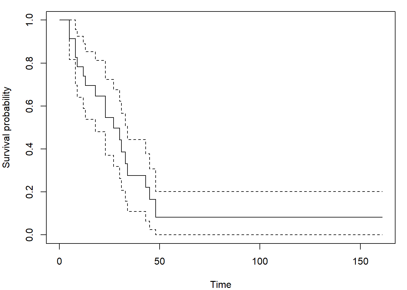
You may also compute and plot confidence intervals for several groups:
fit_grouped <- survfit(Surv(time,status)~x, data=aml, conf.type="plain", conf.int=0.9)
par(mar = c(4,4,1,1))
plot(fit_grouped[1], conf.int=TRUE, col="green", xlab = "Time", ylab = "Survival probability")
lines(fit_grouped[2], conf.int=TRUE, col="magenta")
legend("topright", levels(aml$x), col = c("green","magenta"), lty = 1, bty = "n")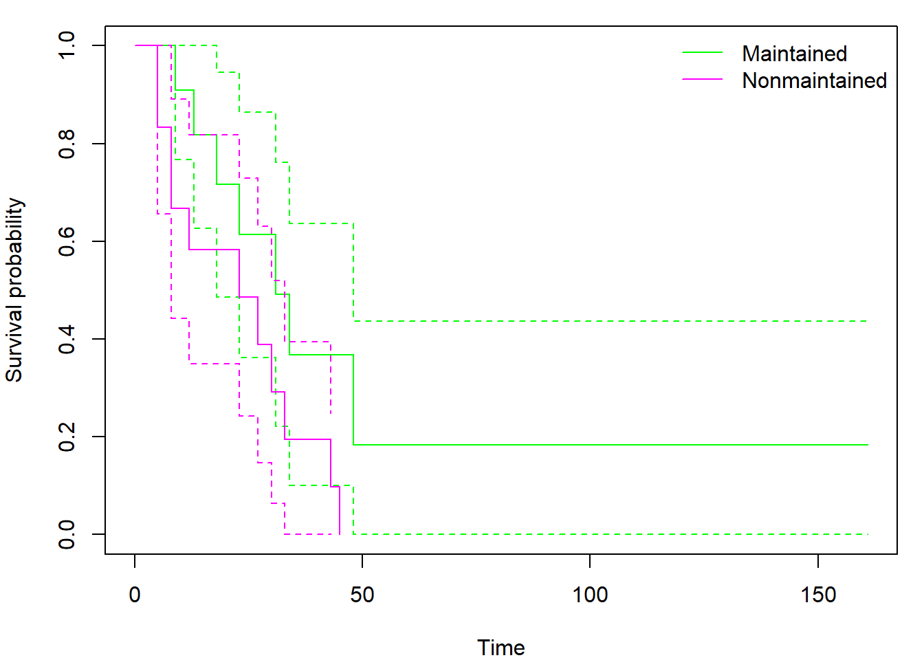
You can also use library(ggplot2) in cooperation with
library(survminer) to obtain nicer plots:
library(survminer)
library(ggplot2)
ggsurvplot(fit_grouped, conf.int = 0.95, censor= F,
ggtheme = theme_minimal())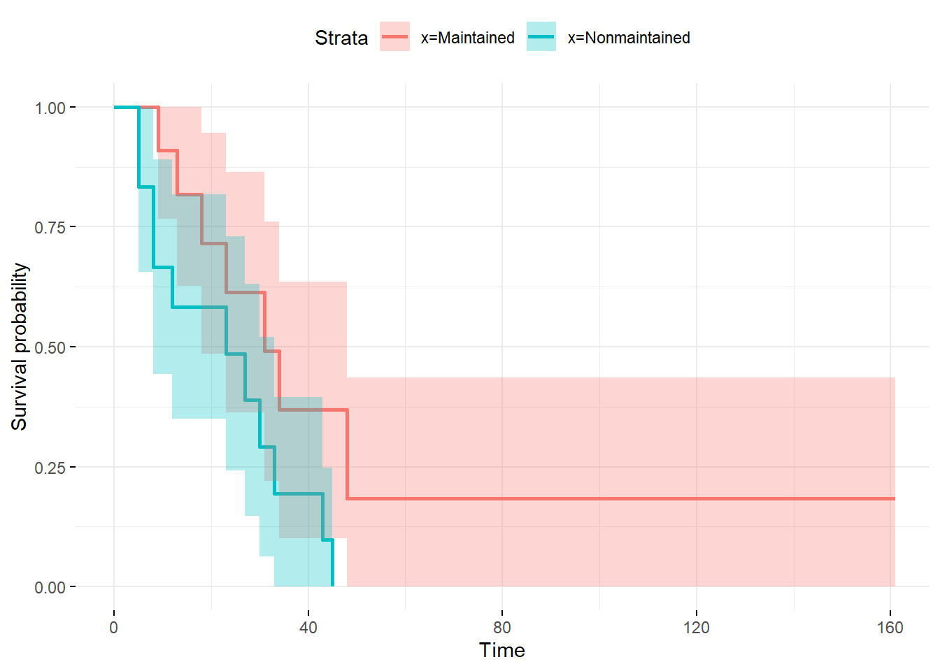 The function
 ggsurvplot inherits the chosen confidence
interval from the survfit object.
Simultaneous confidence bands
There are two different R libraries that can calculate Hall-Wellner simultaneous confidence bands.
1) library(km.ci)
This library includes a function called km.ci, which
requires a survfit object as the input and returns another
survfit object with recalculated lower and
upper components. The output can be processed by any
function that accepts survfit objects – e.g.,
plot, summary, lines.
library("km.ci")
fit <- survfit(Surv(time,status)~1, data=aml, conf.type="plain", conf.int=0.95)
out <- km.ci(fit, conf.level=0.95, tl=5, tu=48, method="hall-wellner")
par(mar = c(4,4,1,1))
plot(out, xlab = "Time", ylab = "Survival Probability")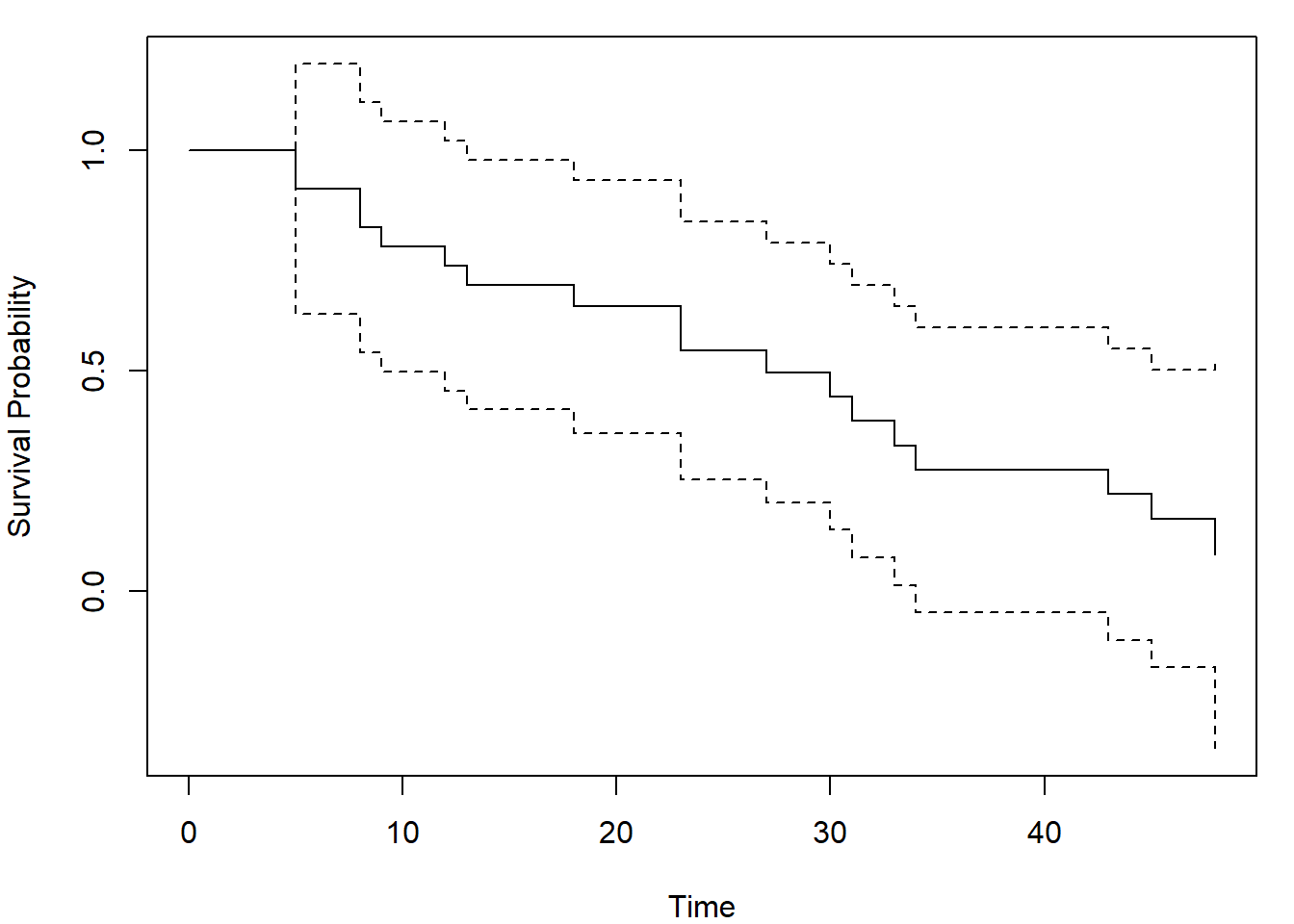
The arguments tl and tu are lower and upper
limits of the interval for which the bands are calculated. Not all
choises of these limits will lead to a useful result, so be careful and
try different inputs. Default values are set to the smallest and largest
event time (tl = min(aml$time[as.logical(aml$status)]) = 5,
tu = max(aml$time[as.logical(aml$status)]) = 48).
Other methods for calculating confidence intervals are the following:
- pointwise:
peto,linear,log,loglog,rothman,grunkemeier, - simultaneous:
hall-werner,loghall,epband,logep.
See Details of km.ci function for explanation of these
abbreviations.
2) library(OIsurv)
This library includes a function called confBands, which
requires a survival object (just Surv) as the input and
returns a list of three vectors (time, lower,
upper). There is a method for plotting lines
from a confBands object, but no method for
plot!
Caution
The library OIsurv has been removed from CRAN. The last
version can still be installed from an archive, e.g. by the command
install.packages("http://www.karlin.mff.cuni.cz/~vavraj/cda/data/OIsurv_0.2.zip", repos =NULL)
## or from github if you use R-version 4.0.0 or higher
library("remotes")
install_github("cran/OIsurv")
Then one can obtain Hall-Wellner confidence bands as follows
library("OIsurv")
out <- confBands(Surv(aml$time,aml$status), confType="plain", confLevel=0.95, type="hall", tU=160)
par(mar = c(4,4,1,1))
plot(fit, xlab = "Time", ylab = "Survival probability", ylim = c(0,1))
lines(out, lty = 3, col = "blue")
legend("topright", c("Kaplan-Meier", "Pointwise confidence interval", "Hall-Werner confidence bands"),
       col = c("black", "black", "blue"), lty = c(1,2,3), bty = "n")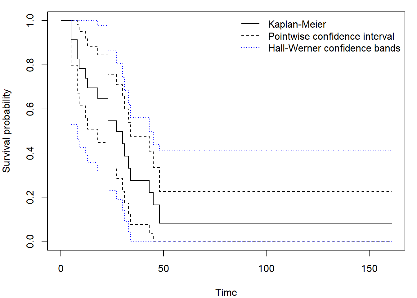
Again be careful when setting minimum tL and maximum
tU time value, the defaults are
tL = min(aml$time)= 5 = first observed or censored time,tU = max(aml$time)= 161 = last observed time.
Only confidence levels confLevel = c(0.9, 0.95, 0.99)
are accepted - default is 0.9!
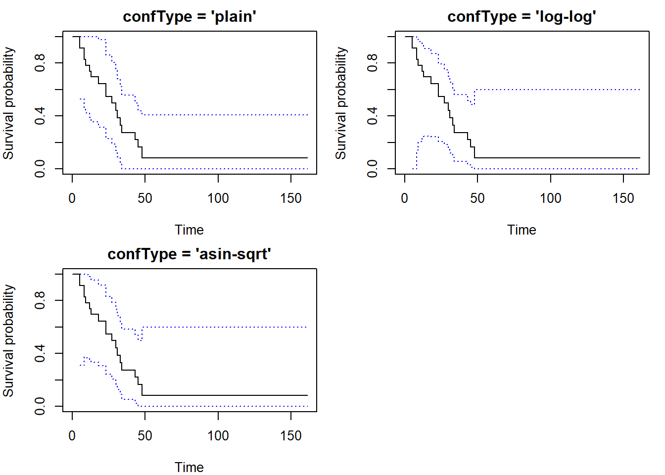
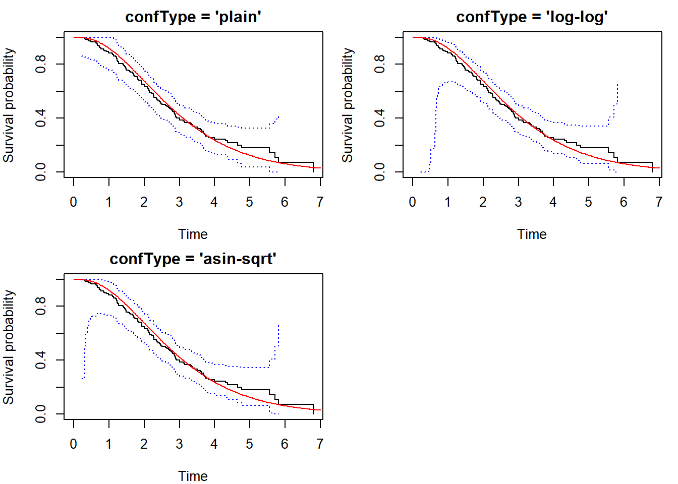
Argument type differentiates between Equal precision
bands ("ep") and Hall-Werner ("hall" or just
"h"). You can also use different versions obtained by
application of Delta theorem:
confType = c("plain", "log-log", "asin-sqrt").
Download the dataset km_all.RData.
The dataframe inside is called all. It includes 101
observations and three variables. The observations are acute lymphatic
leukemia [ALL] patients who had undergone bone marrow transplant. The
variable time contains time (in months) since
transplantation to either death/relapse or end of follow up, whichever
occured first. The outcome of interest is time to death or
relapse of ALL (relapse-free survival). The variable
delta includes the event indicator (1 = death or relapse, 0
= censoring). The variable type distinguishes two different
types of transplant (1 = allogeneic, 2 = autologous).
Calculate and plot the Kaplan-Meier estimate, 95% pointwise confidence intervals and 95% Hall-Wellner confidence bounds for all patients together, for patients with allogeneic transplants, and for patients with autologous transplants.
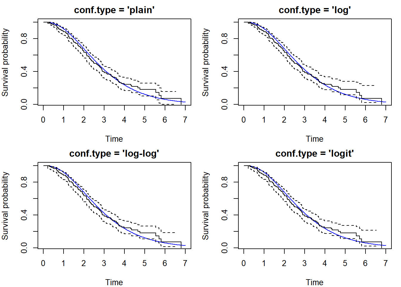
Generate \(n=50\) censored observations as follows: the survival distribution is Weibull with shape parameter \(\alpha=0.7\) and scale parameter \(1/\lambda=2\). Its expectation is \(\Gamma(1+1/\alpha)/\lambda=2\Gamma(17/7)\doteq 2.53\). The censoring distribution is exponential with rate \(\lambda=0.2\) (the expectation is \(1/\lambda=5\)), independent of survival.
Calculate and plot the Kaplan-Meier estimator of \(S(t)\) together with 95% pointwise confidence intervals and 95% Hall-Wellner confidence bounds. Include the true survival function in the plot (use a different color). Include a legend explaining which curve is which and comment on the coverage.
- Deadline for report: Monday 5th December at 9:00
Conduct a simulation study with data created according to Task 2 assignment. Generate such datasets repeatedly and estimate the probability that the true survival curve is wholly covered by the 95% pointwise confidence intervals and 95% Hall-Wellner confidence bounds (restrict the task to a reasonable finite interval).