Building Cox models for censored data (constant covariates)
Jan Vávra
Exercise 7 (13th December 2022)
Theory - the Cox model with time-invariant covariates
We observe \(n\) independent triplets \((X_i, \delta_i, \mathbf{Z}_i), i = 1, \ldots, n\), where
- \(X_i = \min \{T_i, C_i\}\) is censored failure time,
- \(\delta_i = \mathbb{I}_{(T_i \leq C_i)}\) is failure indicator,
- \(\mathbf{Z}_i\) is a vector of covariates.
The Cox model is used to estimate the effect of covariates \(\mathbf{Z}_i\) on continuous (but arbitrary) distribution of failure times \(T_i\) and to test its significance.
In this exercise we will deal with covariates constant in time.
We suppose that the hazard function \(\lambda\) of failure time distribution (assumed to be continuous) given covariates \(T|\mathbf{Z}\) is of the form: \[\lambda(t| \mathbf{Z}) = \lambda_0(t) \exp \left\{ \boldsymbol{\beta}^{\mathsf{T}} \mathbf{Z} \right\},\] where:
- \(\lambda_0(t)\) is the baseline hazard function,
- \(\boldsymbol{\beta} \in \mathbb{R}^p\) is unknown vector of regression coefficients.
Notes:
- See the difference in \(\lambda_0(t)\) (no required shape) compared to \(\lambda_0\) from Exercise 1, see also blackboard notes.
- No intercept included in \(\mathbf{Z}_i\), it is covered by \(\lambda_0(t)\).
- The Cox “proportional hazard” model (under constant covariates) refers to the property of ratio of hazard functions with different covariates:
\[\dfrac{\lambda(t| \mathbf{Z}_1)}{\lambda(t| \mathbf{Z}_2)} = \dfrac{\lambda_0(t)}{\lambda_0(t)} \cdot \dfrac{\exp \left\{ \boldsymbol{\beta}^{\mathsf{T}} \mathbf{Z}_1 \right\}}{\exp \left\{ \boldsymbol{\beta}^{\mathsf{T}} \mathbf{Z}_2 \right\}} = \exp \left\{ \boldsymbol{\beta}^{\mathsf{T}} (\mathbf{Z}_1 - \mathbf{Z}_2) \right\} \quad \text{is constant in time } t.\] Interpretation of \(\beta_j\) coefficient can be derived in the usual way: \[\exp \beta_j = \dfrac{\lambda(t| \mathbf{Z} + \mathbf{e}_j)}{\lambda(t| \mathbf{Z})}.\]
In the case of constant regressors we can express the Cox model in the terms of survival functions:
- \(\Lambda_0(t) = \int \limits_0^{t} \lambda_0(s) \, \mathrm{d} s\) is the cumulative baseline hazard,
- \(S_0(t) = \exp \left\{- \Lambda_0(t) \right\}\) is the baseline survival function,
- general survival function \(S(t|\mathbf{Z})\) is of the form: \[S(t|\mathbf{Z}) = \left[S_0(t)\right]^{\exp \boldsymbol{\beta}^{\mathsf{T}} \mathbf{Z} }.\]
Model is estimated by partial likelihood method that shares properties with classical maximum likelihood method. We can perform tests for:
- single covariates \(\beta_j\): \[\sqrt{n} \dfrac{ \widehat{\beta}_j - \beta_j}{\sqrt{\left(\mathcal{I}_{n}^{-1}\right)_{jj}(\widehat{\boldsymbol{\beta}}, \tau)} } \overset{\mathcal{D}}{\longrightarrow} \mathsf{N}(0,1),\]
- linear combinations of \(\boldsymbol{\beta}\): \[\sqrt{n} \dfrac{ \mathbf{c}^{\mathsf{T}} \widehat{\boldsymbol{\beta}} - \mathbf{c}^{\mathsf{T}} \boldsymbol{\beta} }{\sqrt{\boldsymbol{c}^{\mathsf{T}} \mathcal{I}_{n}^{-1}(\widehat{\boldsymbol{\beta}}, \tau) \boldsymbol{c}} } \overset{\mathcal{D}}{\longrightarrow} \mathsf{N}(0,1),\]
- submodel testing (\(\ell_M (\widehat{\boldsymbol{\beta}})\), \(\ell_S (\widetilde{\boldsymbol{\beta}})\) are maximized partial log-likehoods of model and submodel): \[2 \left( \ell_M (\widehat{\boldsymbol{\beta}}) - \ell_S (\widetilde{\boldsymbol{\beta}}) \right) \overset{\mathcal{D}}{\longrightarrow} \chi_m^2, \quad \text{where } m \text{ is the difference in number of parameters.}\]
We can use the Breslow estimator of cumulative baseline hazard function \[ \widehat{\Lambda}_0(t) = \int \limits_{0}^{t} \dfrac{ \, \mathrm{d} \overline{N}(s)}{\sum \limits_{i=1}^n Y_i (s) \exp \left\{ \widehat{\boldsymbol{\beta}}^{\mathsf{T}} \mathbf{Z}_i \right\}} \] to obtain an estimate of general survival function \[ \widehat{S}(t| \mathbf{Z}) = \exp \left\{ - \widehat{\Lambda}(t| \mathbf{Z})\right\} = \exp \left\{ - \widehat{\Lambda}_0(t) \exp \left\{ \widehat{\boldsymbol{\beta}}^{\mathsf{T}} \mathbf{Z} \right\} \right\}. \]
Obtaining and investigating the dataset
We will work with the dataset pbc contained in the
survival library, see Exercise 1 or help(pbc) for
description.
library(survival)
data(pbc)
variables <- c("id", "time", "status", "trt", "sex", "edema", "bili", "albumin", "platelet")
data <- pbc[, variables]
We will work with the following variables:
| Var. name | Description |
|---|---|
| id | case number |
| status | status at the end of follow-up: 0 = censored, 1 = transplanted, 2 = dead |
| time | number of days of follow-up |
| trt | treatment: 1 = D-penicillamin, 2 = placebo, NA = not randomised |
| sex | sex m/f |
| edema | 0 = no edema, 0.5 = untreated or successfully treated, 1 = edema despite diuretic therapy |
| bili | serum bilirubin (mg/dl) |
| albumin | serum albumin (g/dl) |
| platelet | platelet count |
Here are initial rows of the dataset:
head(data)## id time status trt sex edema bili albumin platelet
## 1 1 400 2 1 f 1.0 14.5 2.60 190
## 2 2 4500 0 1 f 0.0 1.1 4.14 221
## 3 3 1012 2 1 m 0.5 1.4 3.48 151
## 4 4 1925 2 1 f 0.5 1.8 2.54 183
## 5 5 1504 1 2 f 0.0 3.4 3.53 136
## 6 6 2503 2 2 f 0.0 0.8 3.98 NAWe are interested in modelling survival time in untransplanted patients. Patients who had liver transplant will be censored at the moment the transplant was done. Therefore, similarly as in Exercise 1 define \(\delta\) indicator as
data$delta = (data$status == 2)Explorative analysis
First, we will start with explorative analysis using methods we
already know - non-parametric estimation of survival function
(Kaplan-Meier) and logrank test for comparing two (possibly more)
different groups. You can also plot smoothed estimators of hazard
functions (using library(muhaz)) and discuss whether they
seem proportional. The very similar comparison can be made even in terms
of logarithm of Nelson-Aalen estimator of cumulative hazard.
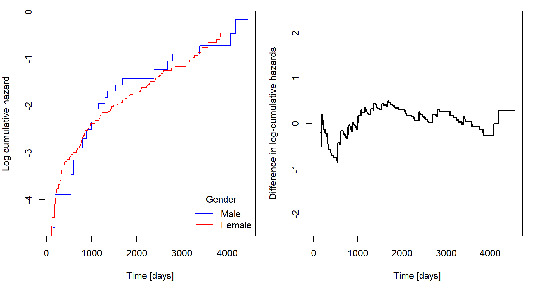
If the proportional hazards assumption holds, then logarithm of cumulative hazard becomes \[ \log( \Lambda(t | \mathbf{Z})) = \log \left( \Lambda_0(t) \cdot \exp \left\{ \boldsymbol{\beta}^{\mathsf{T}} \mathbf{Z} \right\}\right) = \boldsymbol{\beta}^{\mathsf{T}} \mathbf{Z} + \log \Lambda_0(t). \] Which means that the difference of log-cumulative hazard of two individuals is constant in time: \[ \log( \Lambda(t | \mathbf{Z}_1)) - \log( \Lambda(t | \mathbf{Z}_2)) = \boldsymbol{\beta}^{\mathsf{T}} \left( \mathbf{Z}_1 - \mathbf{Z}_2\right). \] Therefore, plotting such difference can be a useful tool for revealing potential problems with satisfying the proportional hazards assumption:
fit <- survfit(Surv(time, pbc$status==2) ~ sex, data = pbc)
lL1 <- log(fit[1]$cumhaz)
lL2 <- log(fit[2]$cumhaz)
# The problem is that each curve is for different time points
# We need to combine them under united times
lcumhaz <- data.frame(lL1 = c(lL1, rep(NA, length(lL2))),
lL2 = c(rep(NA, length(lL1)), lL2),
time = fit$time)
# order data according to time
lcumhaz <- lcumhaz[order(lcumhaz$time),]
# extending the values
last <- c(-Inf, -Inf)
for(i in 1:dim(lcumhaz)[1]){
miss <- is.na(lcumhaz[i,1:2])
lcumhaz[i, which(miss)] <- last[which(miss)]
last <- lcumhaz[i,1:2]
}
# only from the max of min times of each subdata
mintime <- max(sapply(1:2, function(i){min(fit[i]$time)}))
lcumhaz <- lcumhaz[lcumhaz$time >= mintime,]
lcumhaz$difference <- lcumhaz$lL1 - lcumhaz$lL2
par(mfrow = c(1,2), mar = c(4,4,1,1))
plot(lL1 ~ fit[1]$time, col = "blue", type = "s", xlab = "Time [days]", ylab = "Log-cumulative hazard")
lines(lL2 ~ fit[2]$time, col = "red", type = "s")
legend("topleft", c("Male", "Female"), title = "Gender", col = c("blue", "red"), lty = 1, bty = "n")
plot(difference ~ time, lcumhaz, xlab = "Time [days]", ylab = "Difference in log-cumulative hazards",
ylim = c(-1,1)*max(abs(lcumhaz[,1:2]))/2, type = "s", col = "black", lwd = 2)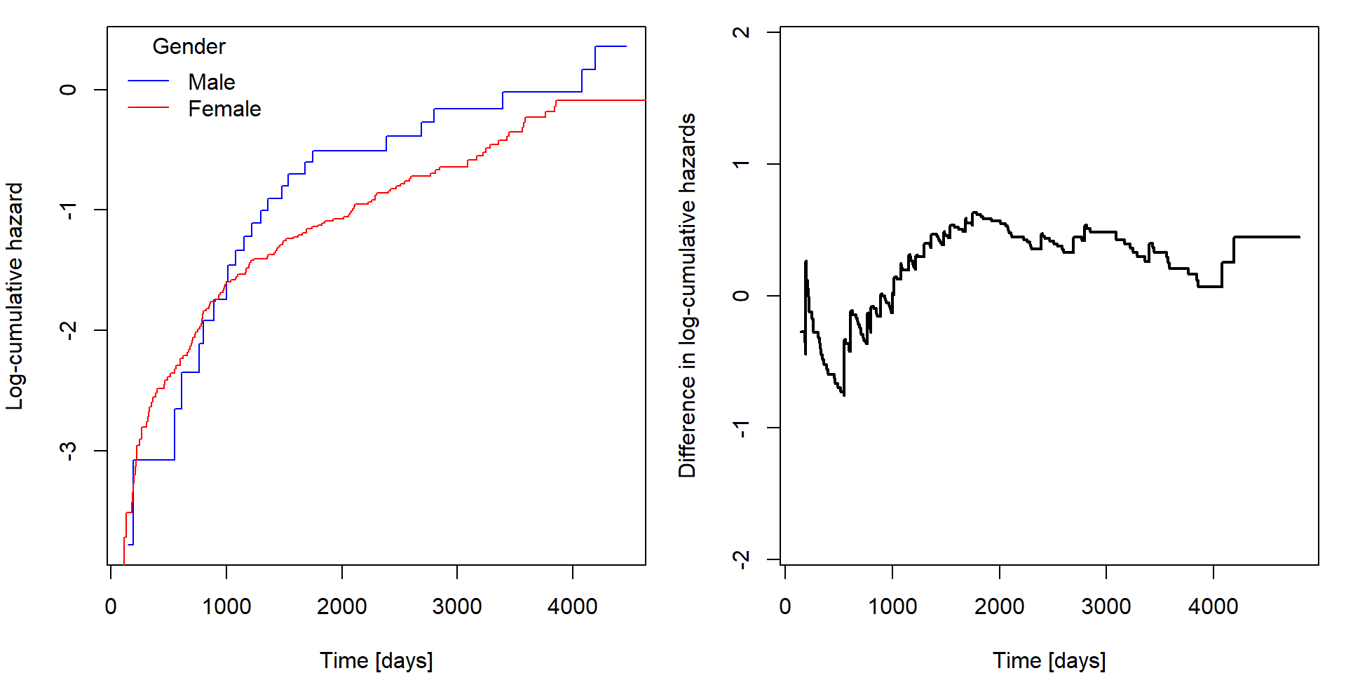 If the black curve is not constant, then the proportional hazards
assumption could by violated with respect to this covariate. In this
case it goes from negative values to positive ones as the curves on the
left cross each other, therefore, the proportionality with respect to
gender may be questioned. However, look only for very serious
violations, otherwise, you would never fit any Cox model as the
difference will not be perfectly constant at any circumstances.
If the black curve is not constant, then the proportional hazards
assumption could by violated with respect to this covariate. In this
case it goes from negative values to positive ones as the curves on the
left cross each other, therefore, the proportionality with respect to
gender may be questioned. However, look only for very serious
violations, otherwise, you would never fit any Cox model as the
difference will not be perfectly constant at any circumstances.
- Choose one binary and one continuous variable.
- Cut continuous variable into two groups (by value “near” median).
- Take binary variable and the created one and perform two-sample analysis.
- Plot survival curves and calculate logrank tests.
- Notice whether the chosen variables look associated with survival.
- Plot estimate of (cumulative) hazard function and try to justify the proportionality assumption of the Cox model with respect to these variables.
An illustration of all possible (read as “not all of them are expected from you”) plots to be supplied (optimization of your code so that it can be easily used for different variables is recommended, but not necessary):
ExplorePBC("chol", type = "continuous", ngroups = 3)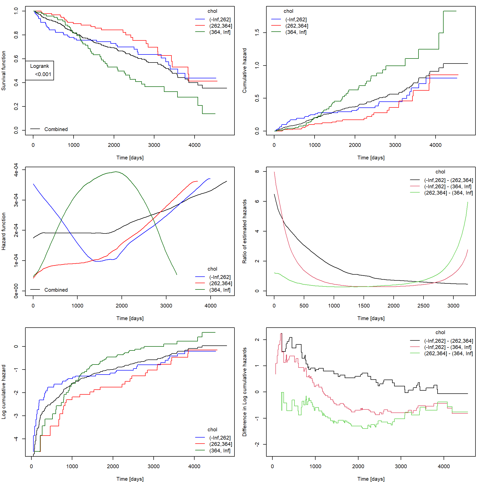
Estimating Cox model
The function to fit the Cox proportional hazards model is called
coxph. It’s syntax is [example]
fit <- coxph(Surv(time, delta) ~ log(age) + chol + hepato, data = pbc)See help(coxph) for additional parameters such as
weights (in case of repeated observations),
na.action (missing-data filter function), ties
(methods for tie handling), …
You can use function summary to view \(\boldsymbol{\beta}\) coefficient estimates
(including exponentiated versions):
summary(fit)## Call:
## coxph(formula = Surv(time, delta) ~ log(age) + chol + hepato,
## data = pbc)
##
## n= 284, number of events= 114
## (134 observations deleted due to missingness)
##
## coef exp(coef) se(coef) z Pr(>|z|)
## log(age) 2.406e+00 1.109e+01 5.231e-01 4.599 4.24e-06 ***
## chol 1.152e-03 1.001e+00 3.134e-04 3.675 0.000238 ***
## hepato 8.941e-01 2.445e+00 2.051e-01 4.358 1.31e-05 ***
## ---
## Signif. codes: 0 '***' 0.001 '**' 0.01 '*' 0.05 '.' 0.1 ' ' 1
##
## exp(coef) exp(-coef) lower .95 upper .95
## log(age) 11.087 0.09019 3.977 30.910
## chol 1.001 0.99885 1.001 1.002
## hepato 2.445 0.40899 1.636 3.655
##
## Concordance= 0.714 (se = 0.023 )
## Likelihood ratio test= 56.08 on 3 df, p=4e-12
## Wald test = 53.26 on 3 df, p=2e-11
## Score (logrank) test = 57.36 on 3 df, p=2e-12Survival probabilities calculation
In our example consider patient of age 50 with hepatomegaly and serum cholesterol 300 mg/dl.
There exists predict.coxph function that seems to be
useful for calculating
type = "lp"- linear predictor,type = "risk"- risk score (exp(lp)),type = "expected"- cumulative hazard function (the expected number of events given the covariates),type = "survival"- survival function,type = "terms"- the terms of the linear predictor.
However, check that you have its new version! The
reference values for baseline used to be means of covariates by default
(even dummy variables used for parametrization of categorical
covariates), see also blackboard notes for
explanation. The type = "expected" setting now works
properly
time.grid <- seq(0, max(pbc$time), length.out = 1000)
baseline <- predict(fit, newdata = data.frame(time = time.grid,
                                              delta = 1,
                                              age = 1,
                                              chol = 0,
                                              hepato = 0),
                    type = "expected")
patient_cumhaz <- predict(fit, newdata = data.frame(time = time.grid,
                                                    delta = 1,
                                                    age = 50,
                                                    chol = 300,
                                                    hepato = 1),
                          type = "expected")

par(mfrow = c(1,2), mar = c(4,4,1,1))
plot(baseline ~ time.grid,
     ylim = c(0,1.8), ylab = "Cumulative hazard function",
     xlab = "Time [days]", type = "l", col = "black", lwd = 2)
lines(patient_cumhaz ~ time.grid, col = "skyblue", lwd = 2)
legend("topleft", c("Baseline", "Patient"),
       col = c("black", "skyblue"), lwd = 2, bty = "n")

plot(exp(-baseline) ~ time.grid,
     ylim = c(0,1), ylab = "Survival probability",
     xlab = "Time [days]", type = "l", col = "black", lwd = 2)
lines(exp(-patient_cumhaz) ~ time.grid, col = "skyblue", lwd = 2)
legend("bottomleft", c("Baseline", "Patient"),
       col = c("black", "skyblue"), lwd = 2, bty = "n")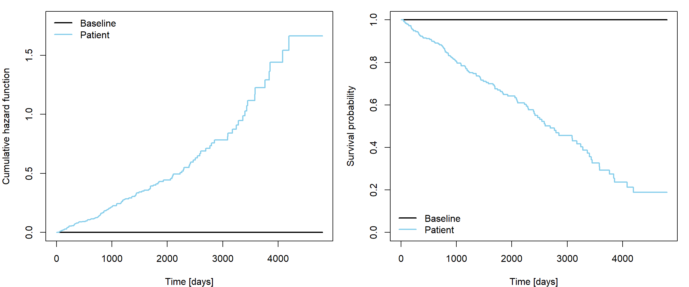
Estimator of baseline cumulative hazard \(\widehat{\Lambda}_0(t)\) can be obtained
using function basehaz with option
centered = F. General cumulative hazard function estimator
can be obtained by combination of basehaz and corresponding
exponentiated linear predictor. Survival function estimator can be
obtained using \(S = \exp \left\{ -
\Lambda\right\}\) transformation:
L0 <- basehaz(fit, centered = F)
# Manual calculation of exp(linear predictor)
patient_LinPred <- sum(c(log(50), 300, 1)*fit$coefficients)
patient_Lambda <- L0$hazard * exp(patient_LinPred)

par(mfrow = c(1,2), mar = c(4,4,1,1))
plot(patient_Lambda~L0$time, type = "s", col = "deepskyblue", xlab = "Time [days]", ylab = "Cumulative hazard")

plot(exp(-patient_Lambda)~L0$time, type = "s", col = "deepskyblue", ylim = c(0,1),
     xlab = "Time [days]", ylab = "Survival probability")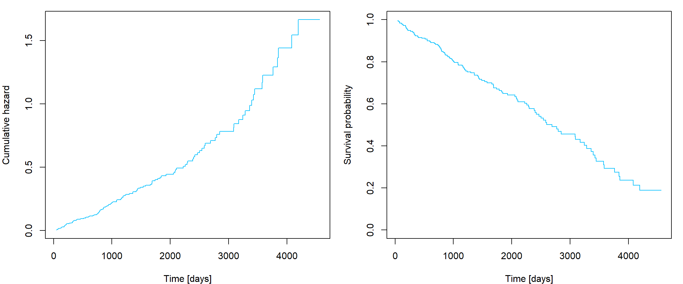
More practical way is to supply newdata to
survfit function applied to fit object (output
of coxph function):
newdata <- data.frame(age = 50, chol = 300, hepato = 1)
fitnew <- survfit(fit, newdata = newdata, conf.type = "plain")

par(mfrow = c(1,2), mar = c(4,4,1,1))
plot(fitnew, fun = "cumhaz", xlab = "Time [Days]", ylab = "Cumulative hazard", col = "deepskyblue", conf.int = F)
plot(fitnew, xlab = "Time [Days]", ylab = "Survival probability", col = "deepskyblue")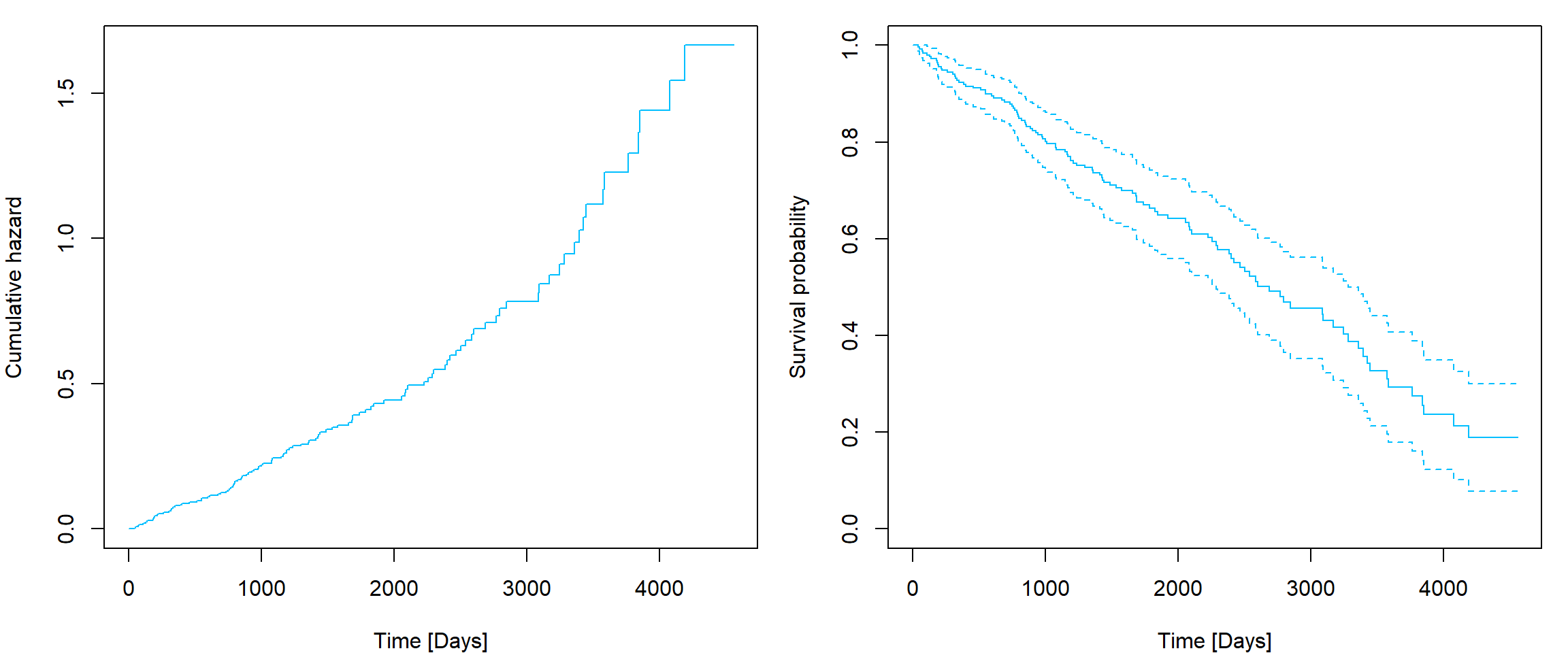
You can use libraries ggplot2 and survminer
to obtain visually nice plots:
library(survminer)
library(ggplot2)

newdata <- with(pbc, data.frame(age =    c( 50,  50,        50),
                                chol =   c(300, 300,       300),
                                hepato = c(  1,   0, 0.5176056)))
fitnew <- survfit(fit, newdata = newdata, conf.type = "plain")

ggsurvplot(fitnew, data = newdata,
           conf.int = TRUE, censor= FALSE,
           legend.labs=c("Patient 1", "Patient 2", "Patient 3"),
           ggtheme = theme_minimal())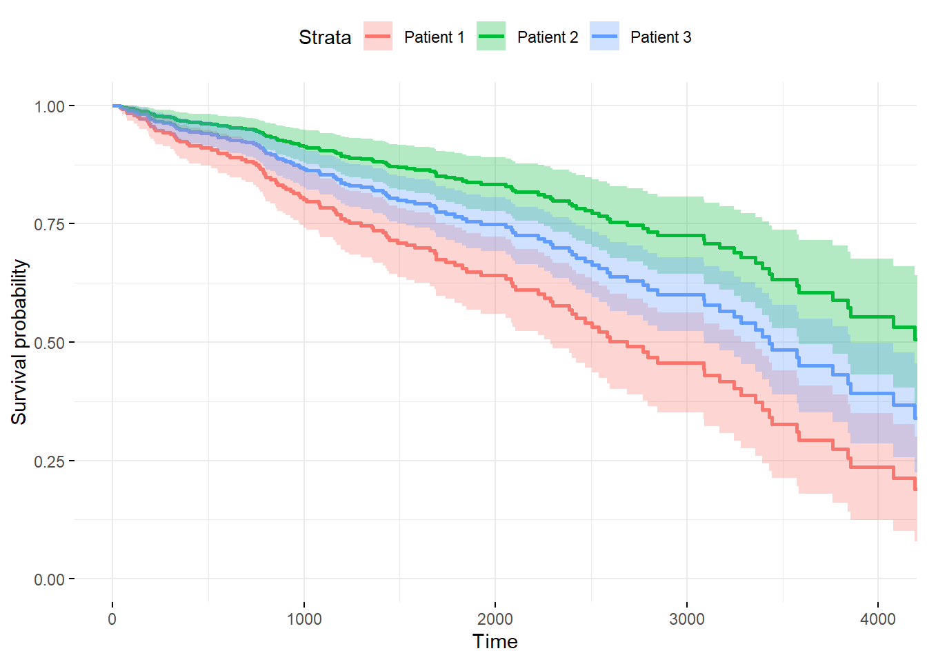
Investigating treatment and bilirubin by Cox model
- Fit the Cox proportional hazards model with treatment as the single covariate.
- Interpret the estimated parameter and its confidence interval.
- Test the hypothesis that treatment has no effect on survival of PBC patients.
- Plot estimated survival functions for both groups based on the Cox model and compare them with Kaplan-Meier estimators of the corresponding two samples.
- Compare the results with the logrank test.
- Fit the Cox proportional hazards model with grouped bilirubin (four groups defined by sample quartiles) as a single covariate.
- Interpret the estimated parameters.
- Test the hypothesis that bilirubin does not affect survival of PBC patients.
- Plot estimated survival functions of these four groups based on the Cox model and compare them with Kaplan-Meier estimators of the corresponding four samples.
- Consider a suitable transformation for continuous bilirubin (for next task).
Cox model with multiple covariates
The logic of specifying the model formula is the same as with
functions lm or glm. Printing the results and
performing tests of hypotheses for model building is also very similar
to other regression functions in R:
summary(fit)
anova(fit)
anova(fit1, fit2)
drop1(fit, test="Chisq")
add1(fit, scope = "bili:trt", test = "Chisq")
The parameter estimation is based on the maximum partial likelihood
method but the asymptotic properties, tests etc. are all the same as
with ordinary likelihood methods. In particular, a submodel is tested
against a wider model by likelihood ratio tests performed by functions
anova or drop1. The difference of
log-partial-likelihoods multiplied by 2 has asymptotically \(\chi^2_m\) distribution if the submodel is
true, where \(m\) is the difference in
the number of parameters. The tests shown in the parameter table of
summary function are Wald tests for zero values of the
individual parameters.
- Build the Cox proportional hazards model for survival of PBC patients.
- Include treatment in the model; consider other variables of interest as additional covariates.
- Continuous variables can be included in the linear form, or after transformation, or in the grouped form.
- Do not include interactions.
- Keep only the covariates that have a significant effect on survival (except treatment).
- Interpret the effect of treatment as well as of other covariates that have been kept in the final model.
- Show confidence intervals for their effects.
- Test their effects on survival of PBC patients.
- Plot estimated survival function depending on the value of treatment (fix reasonably the values of other remaining covariates).
- Compare your final Cox model with your final model from Exercise 1.
- What is the main difference in the model definition and structure?
- Could you plot estimated survival functions for a patient of covariate values of your choice based on these two models?
- Compare the results regarding significance of treatment.
- Is the subset of significant covariates the same as before? Are the chosen parametrizations of covariates the same?
- Any other interesting comparisons?
- Deadline for report: Monday 2nd January at 9:00
Additional material (for your interest only!): Model checking tools
Is there a way to use some residual characteristics and plots for checking the model fit or model asumptions similarly as in linear regression? However, what would be the residuals in this case?
Cox-Snell residuals
If \(T\) is distribution with survival function \(S(t)\) then variable \(-\log S(T)\) follows \(\mathsf{Exp}(1)\) distribution. Which inspires us to use \[\widehat{r}_{i}^{C} = - \log \widehat{S}(X_i | \mathbf{Z}_i).\]
Lagakos residuals (Martingale residuals)
These are defined as \[\widehat{r}_{i}^{L} = \delta_i - \widehat{r}_{i}^{C}\] and their values vary between \(-\infty\) and 1, they have zero mean and are approximately uncorrelated in large samples. Plot them against
- the linear predictor (to validate exponential link),
- any continuous covariate included in the model (to check proper parametrization or validity of proportional hazards assumption),
- any continuous covariate not included in the model (to check its necessity to be included in some form)
and add lowess curve for visualizing the local
behaviour.
Keep in mind that they do not have to be symmetrically distributed around 0 even when the fitted model is correct.
They are the default residuals in coxph output:
fit <- coxph(Surv(time,delta)~log(age)+chol+hepato,data=pbc)
fit$residuals # or use
residuals(fit, type = "martingale")
par(mfrow = c(1,3), mar = c(4,4,1,1))
COL <- c("black", "navyblue")
COLlight <- c("grey", "skyblue")
plot(fit$residuals ~ fit$linear.predictors, xlab = "Linear predictor", ylab = "Martingale residuals",
pch = 21, col = COL[fit$y[,2]+1], bg = COLlight[fit$y[,2]+1])
lines(lowess(fit$residuals ~ fit$linear.predictors), col = "red")
legend("bottomleft", c("Censored", "Observed"), col = COL, pt.bg = COLlight, pch = 21, bty = "n")
plot(fit$residuals ~ model.matrix(fit)[,"log(age)"], xlab = "Log(age)", ylab = "Martingale residuals",
pch = 21, col = COL[fit$y[,2]+1], bg = COLlight[fit$y[,2]+1])
lines(lowess(fit$residuals ~ model.matrix(fit)[,"log(age)"]), col = "red")
legend("bottomleft", c("Censored", "Observed"), col = COL, pt.bg = COLlight, pch = 21, bty = "n")
plot(fit$residuals ~ log(pbc[complete.cases(pbc[,c("time","delta","age","chol","hepato")]),"bili"]),
xlab = "Log(bili) [log(mg/dl]", ylab = "Martingale residuals",
pch = 21, col = COL[fit$y[,2]+1], bg = COLlight[fit$y[,2]+1])
lines(lowess(fit$residuals ~ log(pbc[complete.cases(pbc[,c("time","delta","age","chol","hepato")]),"bili"])),
col = "red")
legend("bottomright", c("Censored", "Observed"), col = COL, pt.bg = COLlight, pch = 21, bty = "n")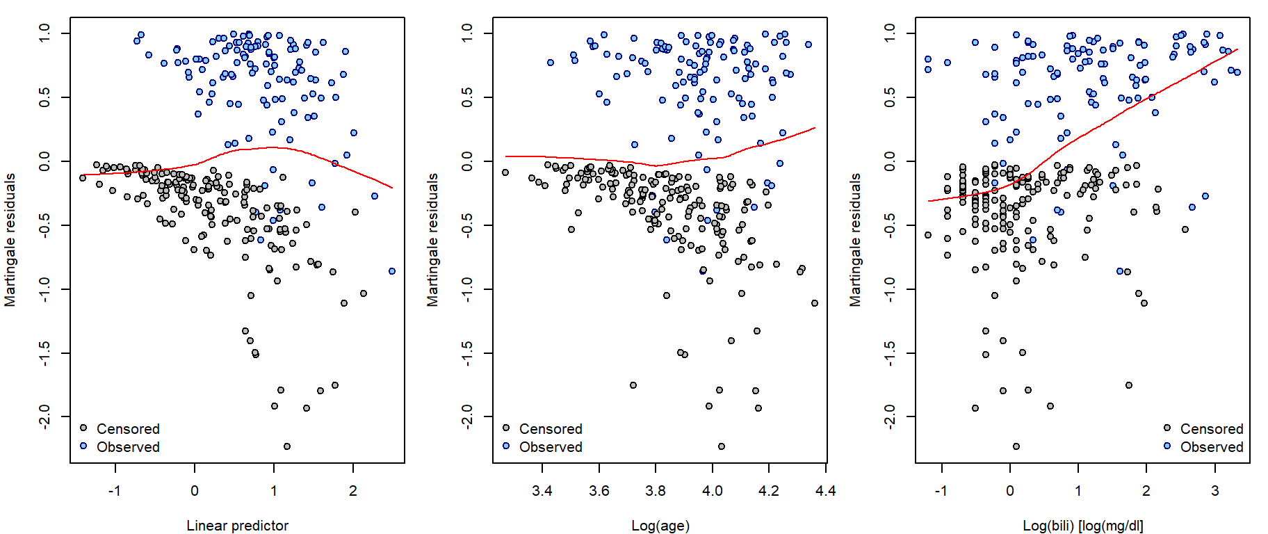
Deviance residuals
These residuals are result of symmetrization of Lagakos residuals:
\[\widehat{r}_i^D
= \mathrm{sign} (\widehat{r}_i^L) \sqrt{- 2 \left[ \widehat{r}_i^L +
\delta_i \log \left( \delta_i - \widehat{r}_i^L \right) \right]}
= \mathrm{sign} (\widehat{r}_i^L) \sqrt{- 2 \left[ \widehat{r}_i^L +
\delta_i \log \widehat{r}_i^C \right]}\]
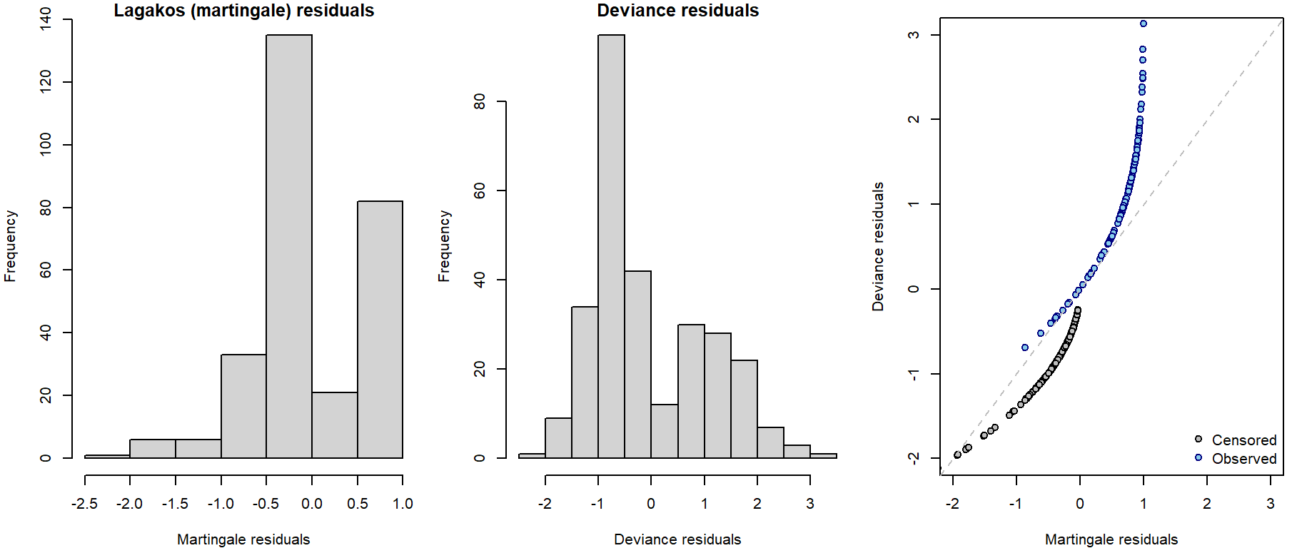
They are called deviance residuals due to their connection to model deviance (scaled difference of log-(partial)-likelihoods under current model of investigation \(\widehat{L}_c\) and the full saturated model \(\widehat{L}_f\)): \[D = -2 \left[ \log \widehat{L}_c - \log \widehat{L}_f \right] = \sum \limits_{i=1}^{n} \left( \widehat{r}_i^D \right)^2\] Although being symmetrically distributed around zero, they do not necessarily sum up to zero. Can be used similarly as Lagakos residuals:
residuals(fit, type = "deviance")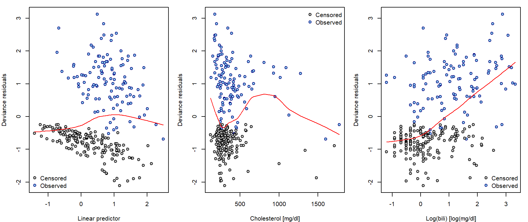
Checking the PH assumption
Remember, that under proportional hazards (PH) assumption it holds that \[ \Lambda(t|\mathbf{Z}) = \Lambda_0(t) \exp \left\{ \boldsymbol{\beta}^{\mathsf{T}} \mathbf{Z} \right\}, \quad \text{which implies} \quad \log \Lambda(t|\mathbf{Z}) = \log \Lambda_0(t) + \boldsymbol{\beta}^{\mathsf{T}} \mathbf{Z}. \] Therefore, a difference of two such transformed curves should be a constant function in time: \[ \log \Lambda(t|\mathbf{Z}_1) - \log \Lambda(t|\mathbf{Z}_2) = \boldsymbol{\beta}^{\mathsf{T}} \left( \mathbf{Z}_1 - \mathbf{Z}_2 \right). \]
However, we cannot directly use the estimated survival
curves based on coxph output as this difference will be
always constant. We need to perform stratification
which is a generalization that allows \(K\) different baseline hazard functions
\(\lambda_{0,k}\) in \(K\) strata defined by some of the
covariates. If the PH assumption is violated, this is one of the
possible ways to deal with it.
fit <- coxph(Surv(time,delta)~log(age)+chol+hepato+strata(sex),data=pbc)
cumhaz <- basehaz(fit)
# now contains 3 columns: cumhazard, time and stratification according to selected factor variable
Now we can perform similar calculations as in explorative analysis. However, now the estimates of log-cumulative hazard are adjusted for effects of other covariates. Notice that the plots seem to be the same as in explorative analysis, but they are not, just very similar:
 My own implementation of this method using stratification according to
one selected covariate and some fitted
My own implementation of this method using stratification according to
one selected covariate and some fitted coxph model:
check.coxph <- function(fit, var, type, ngroups = 2, koef = 1.1,
  COL = c("blue", "red", "darkgreen", "darkviolet", "orange", "skyblue", "pink", "lawngreen"))
{
  # fit is coxph object without stratification
  if(type == "continuous"){
    qq = quantile(pbc[,var], probs = seq(0,1,length.out = ngroups+1), na.rm = T)
    ff = cut(pbc[,var], breaks = c(-Inf, qq[2:ngroups], Inf))
  }else{
    ff = factor(pbc[,var])
  }
  nlevff <- nlevels(ff[!is.na(ff)])

  ### update the fit by adding strata
  fits <- coxph(as.formula(paste0(as.character(fit$formula[2]),
                                  " ~ ",
                                  as.character(fit$formula[3]),
                                  " + strata(ff)")), data = pbc)
  cumhaz <- basehaz(fits)

  lcumhaz <- data.frame(time = cumhaz$time)
  TAB <- table(cumhaz$strata)
  for(i in 1:nlevff){
    if(i > 1){
      nrep1 <- sum(TAB[1:(i-1)])
    }else{
      nrep1 = 0
    }
    if(i < nlevff){
      nrep2 <- sum(TAB[(i+1):nlevff])
    }else{
      nrep2 = 0
    }
    lcumhaz[,paste0("lL",i)] <- c(rep(NA, nrep1),
                                  log(cumhaz$hazard[cumhaz$strata == levels(ff)[i]]),
                                  rep(NA, nrep2))
  }

  # order data according to time
  lcumhaz <- lcumhaz[order(lcumhaz$time),]
  # extending the values
  last <- rep(-Inf, nlevff)
  for(i in 1:dim(lcumhaz)[1]){
    miss <- is.na(lcumhaz[i,paste0("lL",1:nlevff)])
    lcumhaz[i, which(miss)+1] <- last[which(miss)]
    last <- lcumhaz[i,paste0("lL",1:nlevff)]
  }

  maxs <- sapply(1:nlevff, function(i){max(abs(lcumhaz[is.finite(lcumhaz[,paste0("lL",i)]),paste0("lL",i)]))})

  # Log-cumulative hazards by strata
  par(mfrow = c(1,2), mar = c(4,4,1,1))
  plot(log(cumhaz$hazard) ~ cumhaz$time, col = "blue",
       xlab = "Time [days]", ylab = "Log cumulative hazard", type = "n",
       ylim = range(log(cumhaz$hazard)))
  for(i in 1:nlevff){
    lines(log(cumhaz$hazard[cumhaz$strata==levels(ff)[i]]) ~ cumhaz$time[cumhaz$strata==levels(ff)[i]], col = COL[i], type= "s")
  }
  legend("bottomright", levels(ff), col = COL, lty = 1, title = var, bty = "n")


  ymax <- -Inf
  for(i in 1:(nlevff-1)){
    for(j in (i+1):nlevff){
      difs <- abs(lcumhaz[,paste0("lL",i)] - lcumhaz[,paste0("lL",j)])
      ymax <- max(ymax, max(difs[is.finite(difs)]))
    }
  }

  # Differences between log-cumulative hazards of different strata
  plot(lcumhaz$lL1 - lcumhaz$lL2 ~ lcumhaz$time,
       xlab = "Time [days]", ylab = "Difference in Log cumulative hazards",
       ylim = c(-1,1)*ymax*koef, type = "n", col = "black", lwd = 2)
  count = 0
  leg <- c()
  for(i in 1:(nlevff-1)){
    for(j in (i+1):nlevff){
      count <- count + 1
      leg <- c(leg, paste0(levels(ff)[i], " - ", levels(ff)[j]))
      lines(lcumhaz[,paste0("lL",i)] - lcumhaz[,paste0("lL",j)] ~ lcumhaz$time, col = count, type = "s")
    }
  }
  legend("topright", leg, title = var, col = 1:count, lty = 1, bty = "n")
}


fit <- coxph(Surv(time,delta)~log(age)+chol+hepato,data=pbc)

#check.coxph(fit, var = "age", type = "continuous", ngroups = 3)
#check.coxph(fit, var = "albumin", type = "continuous", ngroups = 3)
#check.coxph(fit, var = "alk.phos", type = "continuous", ngroups = 3)
#check.coxph(fit, var = "ast", type = "continuous", ngroups = 3)
check.coxph(fit, var = "bili", type = "continuous", ngroups = 3)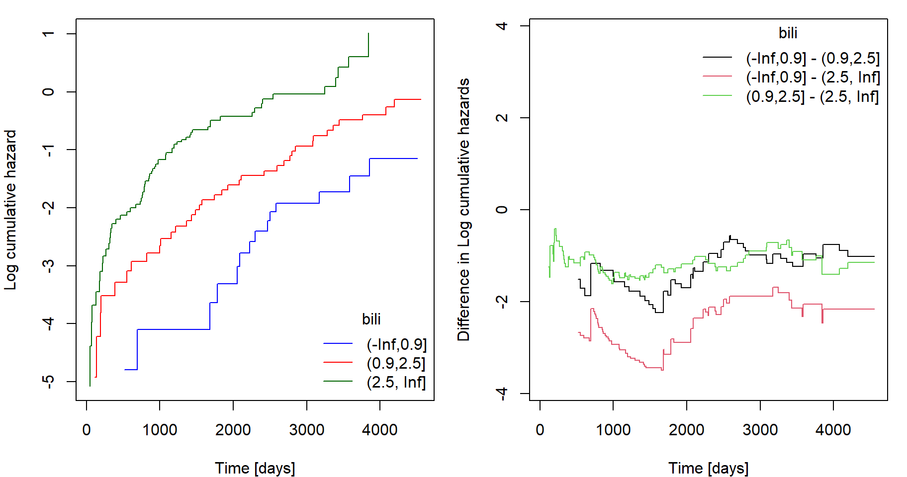
#check.coxph(fit, var = "chol", type = "continuous", ngroups = 3)
#check.coxph(fit, var = "copper", type = "continuous", ngroups = 3)
#check.coxph(fit, var = "platelet", type = "continuous", ngroups = 3)
#check.coxph(fit, var = "protime", type = "continuous", ngroups = 3)
#check.coxph(fit, var = "trig", type = "continuous", ngroups = 3)

#check.coxph(fit, "ascites", type = "categorical")
#check.coxph(fit, "hepato", type = "categorical")
#check.coxph(fit, "spiders", type = "categorical")
#check.coxph(fit, "sex", type = "categorical")
#check.coxph(fit, "trt", type = "categorical")
#check.coxph(fit, "edema", type = "categorical")